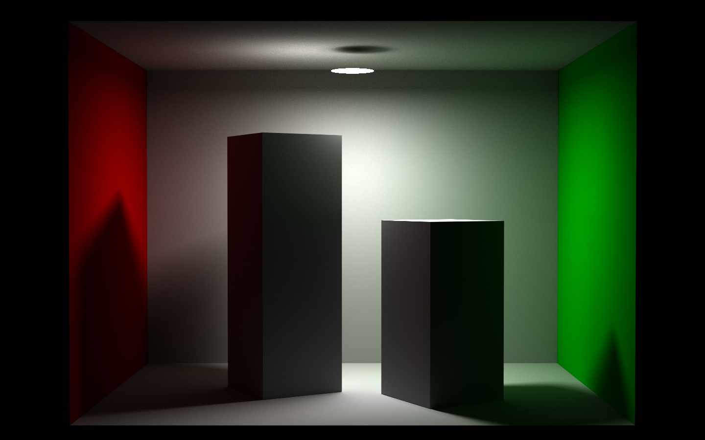
I tried path tracing two years ago in my ray tracer. However without taking some notes, I’ve already forgotten almost everything about it. Recently I reviewed the theory and the code, picked up something from it. I’d like to take some notes so that I can get it immediately next time I forget it. Before everything, here is a Cornell box scene rendered with path tracing:

I really want to render something different using my ray tracer, however it doesn’t have a GUI editor so far. Everything is through script and editing a scene through script is really a painful experience. I do plan to add GUI support using QT, however I don’t have time for it these days. Hopefully I will have some time in the near future.

What is Path Tracing

There are quite a lot of global illumination algorithms around. Radiosity is usually used to generate light map, I have briefly mentioned it in my previous blog post. However it fails to deliver correct result if mirror-like or highly glossy materials are present in the scene. Irraidiance cache is another kind of algorithm that simulates diffuse reflections between surfaces, it also captures effects like color bleeding, but fails when there is specular surfaces. Photon mapping can adapts well to those specular surfaces and it can also catch effects like color bleeding, it can even generate beautiful caustics. Although photon mapping is consistent, it is not unbiased.

Path tracing is a type of ray tracing algorithm which solves the rendering equation very well. And it is unbiased and consistent which means that as the number of samples increases per-pixel, the result is heading for the physically correct value. It is simple and easy to implement once you have mastered the math behind it. Here is the simplest path tracing algorithm implementation I’ve ever seen, only 99 lines of C++. Although it is small, it has everything, soft shadow, caustics, color bleeding, reflection and refraction and it is even multi-threaded.

A whitted ray tracing only handles reflection of one bounce. A path tracing extends it by generating paths recursively so that it accounts light contribution of any bounces instead of just one bounce. Effects like color bleeding requires at least light of two bounces. So it won’t be available in a whitted ray tracing. There are several questions to be answered:

• What is the math behind it?
• How to generate the path with specific number of bounces?
• How to generate infinite number of paths with finite resources of computation?

Math behind it

Basically every algorithm tries to simulate the famous rendering equation. It is also a good start point for path tracing theory.

$$ {L_{o}(\omega_{o}) = L_{e}(\omega_{o}) + \int L_{i}(\omega_{i}) *f( \omega_{i}, \omega_{o} ) *cos(\theta_{i}) d\omega_{i}} $$

The difficulty for simulating this equation is that L is appeared at both side of the equation. And L itself is a function of position and direction, that said the L at different side of this equation may have different values, most of the time they are not the same. In order to compute the Lo on the left, it is necessary to get the radiance values for Li first. Notice that we may need multiple Li since it is an integral. Actually Lo is no essentially different from Li, they are all radiance values. So … in order to generate the Li, we need other radiance values which is implicit in this equation. And it is a recursive problem, never ends. That is why rendering equation is very hard to solve.

We are now rewriting this equation removing the difference between Lo and Li, they are all L

$$ {L(\omega_{o}) = L_{e}(\omega_{o}) + \int L(\omega_{i}) * f( \omega_{i}, \omega_{o} ) *cos(\theta_{i}) d\omega_{i}} $$

In order to make it more clear for paths with different number of bounces, let’s redefine the L and brdf this way:

$$ {L(\omega) = L( x_{0} \to x_{1} )} $$

The left L means that radiance value along the direction $ {\omega} $ , while the right one represents the radiance value from point x0 to x1.

$$ {f( \omega_{i}, \omega_{o} ) = f( x_{0} \to x_{1} \to x_{2} ) } $$

This one is similar. The left one is the traditional four-dimensional brdf, the right one is the brdf value at point x1, the two directions are determined by point x0 and x2.

Now it is the time to expand the equation. Replace the radiance value on the right with the equation itself. For any path, let’s define the first vertex is $ x_0 $ , the second one is $ x_1 $ and so on. $ \theta_1 $ stands for the angle between surface normal and the direction pointing from $ x_1 $ to $ x_2 $ . $ {\omega_{1}}$ is the solid angle around the point $ x_1 $.

$$ {L(x_{1} \to x_{0}) = L_{e}(x_{1} \to x_{0}) + \int L(x_{2} \to x_{1}) * f( x_{2} \to x_{1} \to x_{0} ) *cos(\theta_{1}) d\omega_{1}} $$

Although we redefined rendering equation this way, we are still integrating over the solid angle instead of area because that’s exactly how we generate path later. If we replace the L value on the right with the equation itself, we have something like this:

$ \begin{array} {lcl} L(x_{1} \to x_{0}) & = & L_{e}(x_{1} \to x_{0}) + \int (L_{e}(x_{2} \to x_{1}) + \\ & & \int L(x_{3} \to x_{2}) * f( x_{3} \to x_{2} \to x_{1} ) *cos(\theta_{2}) d\omega_{2}) * f( x_{2} \to x_{1} \to x_{0} ) *cos(\theta_{1}) d\omega_{1} \\ & = & L_{e}(x_{1} \to x_{0}) + \\ & & \int L_{e}(x_{2} \to x_{1}) * f( x_{2} \to x_{1} \to x_{0} ) *cos(\theta_{1}) d\omega_{1} + \\ & & \int \int L(x_{3} \to x_{2}) * f( x_{3} \to x_{2} \to x_{1} ) *cos(\theta_{2}) * f( x_{2} \to x_{1} \to x_{0} ) *cos(\theta_{1}) d\omega_{1}d\omega_{2} \end{array} $

It is a very long equation. The simple truth here is that it represents 0 bounces contribution (intersected object is emissive) in the third line of this equation, 1 bounce in the fourth line of it and further bounces in the last line. Maybe expend it again will be more clear, however I don’t think I can show that long a equation in such small space. In case it is too long, let’s define some basic terms first.

It is not hard to get the light contribution of n bounces, n is from 1 to infinite.

$$ P(n) = {\int...\int} L_{e}(x_{n+1} \to x_{n}) * \prod\limits_{i=1}^n (f( x_{i+1} \to x_{i} \to x_{i-1} ) *cos(\theta_{i})) d\omega_{1}d\omega_{2}...d\omega_{n} $$

With the above equations replacing the extended rendering equation, we have a quite simpler form.

$$ { L(x_{1} \to x_{0}) = L_{e}(x_{1} \to x_{0}) + \sum\limits_{n=1}^{\infty} P(n) } $$

That is the exact form we used to simulate rendering equation with path tracing. What it says is relatively clear comparing with the original rendering equation, radiance from a specific point to another is the summation of the emissive energy and the light contribution with every number of bounces. That leaves us only two problems to solve.

Generate a path with specific number of bounces

Now we are focusing on P(n). With Monte Carlo, we only need to generate a number of paths with n time bounces to simulate the integral. Given a specific number “n”, how to generate a path with the exact number of bounces. The answer is you can randomly pick the points anywhere you want with any probability density function(pdf), however different form of rendering equation is needed if picking point through surfaces instead of solid angle. I never seen any path tracing implementation picking sample points on surfaces, may be you can do that in cornell case. However it will introduce high variance for a moderate scene. Although PBRT does start the theory with this way, it ends up to generate path through brdf eventually.

The first point is determined by your camera ray, it is fixed. To generate the second point, we need to sample a direction from the first point. Again, there are infinite number of pdf. The rule is that the more the pdf looks like the function to be integrated, which is the multiplication of brdf, cosine and radiance in this case, the faster it converges to accurate result. This is importance sampling. Actually switching from sampling surfaces to sampling solid angle is already some kind of importance sampling, because it increases the chances of non-zero contribution paths.

The issue here is that we have totally no idea on what the distribution of radiance is almost all time. There is no way to generate a pdf that is similar to the function to be integrated. Typically sampling a direction by a cosine-weighted pdf works pretty well in practice. Special care needs to be paid for delta surfaces, like mirror. After sampling a direction, it is easy and straight forward to find the second point in the path we are looking for. And then repeat the process again and again until you have n-1 vertices in your path.

For the last vertex, it should be exactly on a light surface. This time sampling a point on light surfaces is better than sampling brdf alone because sampling brdf will probably miss the light. Of course that’s for diffuse surfaces. For delta surfaces or highly glossy surfaces, sampling a brdf will be better.

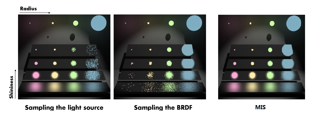
Here is an example taken from here. The image on the left samples light source, the glossier the surface is, the worse the result is. As for the middle one which samples brdf, we can see there is extremely low convergence rate for small light sources. The right most one uses multiple importance sampling, it gives pretty good result. And for the best part, you don’t even need to know which pdf is similar to the integrated function, it just works.

Sampling infinitive number of paths with finite resources

We have only one question left, how to generate result for infinitive number of bounces. Russion roullete is the key here.

$$ { L(x_{1} \to x_{0}) = L_{e}(x_{1} \to x_{0}) + \sum\limits_{n=1}^{\infty} P(n) } $$

Since it is assumed that the more bounces in the path, the less contribution it has to the final image. There are cases breaking this assumption for sure, however it is true most of the time. If we define a function like this:

$$ P^{'}(n)= \begin{cases} \frac{P(n)}{T}&:t<T \\ 0&:t\ge T \end{cases} $$

We have certain probability to terminate the path without introducing any bias. Putting this into the rendering equation:

$$ { L(x_{1} \to x_{0}) = L_{e}(x_{1} \to x_{0}) + P(0) + P(1) + P(2) + \sum\limits_{n=3}^{\infty} P^{'}(n) } $$

It seems look better, however it is still needed for infinite number of paths to generate the result. Let’s go further:

$$ { L(x_{1} \to x_{0}) = L_{e}(x_{1} \to x_{0}) + P(0) + P(1) + P(2) + \frac{1}{T} * ( P(3) + \frac{1}{T} * ( P(4) + \frac{1}{T} * ( P(5) + ... ))) } $$

We have non-zero probability of reaching path with any number of bounces. In a practical case, it will most likely to terminate the whole computation after several number of bounces without introducing any bias in the rendering equation.

Optimization

Path tracing is an elegant algorithm, it captures all effects in the rendering equation. However it usually takes a great number of samples per pixel to reach acceptable result, that means a lot of time consumed by computing. There are a couple of ways to improve the performance of path tracing.

Reuse Generated Path

There is totally no need to regenerate path from scratch for paths with different number of bounces. One can generate a path with russion routtele and reuse each vertex multiple times. Usually only one path is generated for each pixel sample, you can compute result for P(1), P(2), P(3) if you have a path of three bounces. Of course you can have multiple sample per pixel.

Multi-threaded Optimization

Instead of modifying the algorithm itself, hardware resources are also valuable if used well. So I implemented multi-threading ray tracing to accelerate the whole process. The general idea is quite simple, divide the image into a number of tiles of the same size. Generate a task for each tile and push it into a task queue. Each thread picks a task once it is idle. If the queue is empty, it just terminates itself. The number of tiles should not be exactly the same with the number of thread allocated for best performance because some of them may idle if they finish their task first.

It turned out a simple multi-threading model will boost the performance by more than five times on my Intel CPU, which is Xeon(R) E3-1230 v3.

Reference

[1] Physically Based Rendering, second edition
[2] Bias in Rendering
[3] smallpt: Blobal Illumination in 99 lines of C++
[4] Robust Monte Carlo Method for Light Transport Simulation