A couple of days ago, an artist asked me what exactly a directional light map is. I found this page talking about the solutions in Unity 3D and explained to him. And I am reading the book “Real time rendering“ these days, it also talks about directional light map, which gives a more detailed and low-level explanation on it. Sounds like a very interesting topic, so I decided to take some notes.

Although directional light map is nothing new, it is widely used in multiple commercial game engines, like Unreal Engine, Unity 3D and Source Engine. It is an advanced version of classical light map that everyone knows about. Traditional light map won’t consider normal map variance, which leads to very flat and diffuse look on surfaces. Directional light map tries to solve the problem by baking more information so that it will take normal map into account.

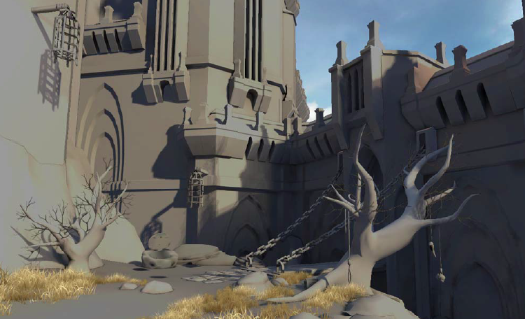
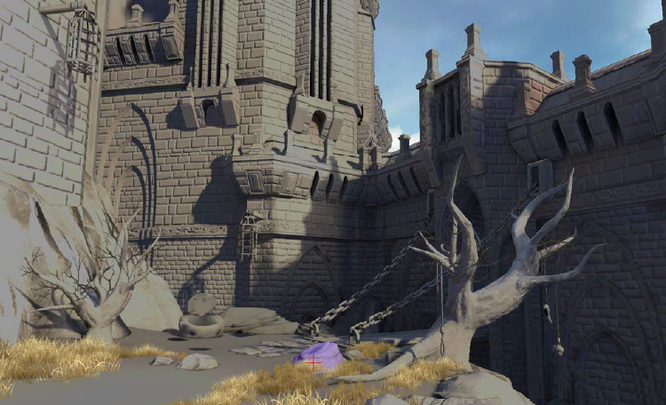
Left image shows the old light map technique. Right image demonstrates how directional light map can greatly enhance visual quality. As we can see from the two, it is apparent that directional light map shows more detail than a light map does.

What exactly is a light map from the perspective of mathematics. The answer is quite simple, it stores irradiance values for each sampled location on surface. Instead of talking about directional light map alone, I decided to start from the very basic, the rendering equation. Hopefully it will gives the reader a more low-level and mathematics interpretation and a deeper understanding of this method.

Light Map

Rendering Equation

Basically everything in computer graphics, whether it is offline rendering or real time rendering, tries to simulate the famous rendering equation. The only difference is that how much assumption it has to make to design the algorithm. Some places little limitation, like path tracing. Some puts more, like ambient occlusion. The less assumption it is made, it is more likely to achieve better result.

$$ {L_{o}(\omega_{o}) = \int L_{i}(\omega_{i}) *f( \omega_{i}, \omega_{o} ) *cos(\theta_{i}) d\omega_{i}} $$

In certain cases, you may have a Le component in this equation, which represents emissive materials. Since it is not involved in the context of this article, it is not shown here. Li and Lo represent radiance value for the output and input angle. “f” is the four dimensional brdf function. $\theta_{i}$ is the angle between $ \omega_{i} $ and normal. Don’t be afraid of this integral, what it says is to accumulate contributions of light from all angles, nothing more.

For traditional light map, there are a couple of assumptions made:

• All surfaces in the scene is purely diffuse which behaves as exactly lambertian surfaces.
• All objects are static.
• All lights are static.

For a scene like this, no light will change if the viewing angle is different across frames. That said we can totally bake all lighting information into textures in a pre-process step and use these textures for real time rendering. Those textures are the light map. They were first used in Quake. The question is in what form the lighting information should be stored in light map. We will answer the question in the following sections.

Radiance and irradiance

Here are a couple of basic terms in computer graphics:

• Flux. Energy that passes through a specific area per-time.
• Irradiance. Flux per unit-area
• radiance. Flux per unit-area per solid angle

It is radiance that human can perceive and its value is not changed along a certain direction if there is only vacuum. The following equation demonstrates how to get irradiance value from radiance:

$$ { E = \int L_{i}(\omega_{i}) *cos(\theta_{i}) d\omega_{i}} $$

Lambertian surface feature

Lambertian surface appears equally bright from all viewing directions and reflects all incident light. It has a very nice feature, the brdf function returns a constant value regardless of the two angles for any specific position. The below equation is the directional-hemisphere reflectance equation:

$$ \rho_{d} = \int f( \omega_{i}, \omega_{o} ) *cos(\theta_{i}) d\omega_{i} $$

Notice that $ \rho_{d} $ is a function of position. Since we are focusing on a single position, it is dropped in the above equation. Because brdf is a constant value, we have the following equation after isolating this factor out of the integral:

$$ \rho_{d} = f( \omega_{i}, \omega_{o} ) * \int cos(\theta_{i}) d\omega_{i} $$

The integral component is actually $ \pi $ :

$$ \begin{array} {lcl} \int cos(\theta_{i}) d\omega_{i} & = & \int_{0}^{2\pi} \int_{0}^{\frac{\pi}{2}} cos(\theta_{i}) sin(\theta_{i}) d\theta_i d\phi \\\\ & = & \int_{0}^{2\pi} d\phi \int_{0}^{\frac{\pi}{2}} cos(\theta_{i}) sin(\theta_{i}) d\theta_i \\\\ & = & 2\pi \int_{0}^{\frac{\pi}{2}} cos(\theta_{i}) sin(\theta_{i}) d\theta_i \\\\ & = & 0.5 * \pi \int_{0}^{\frac{\pi}{2}} sin(2\theta_{i}) d(2\theta_i) \\\\ & = & \pi \end{array} $$

So we have the final equation for our lambertian brdf, which is extremely simple:

$$ f(\omega_{i}, \omega_{o}) = \dfrac{\rho_{d}}{\pi} $$

If we substitute the brdf function in the rendering equation with this one, here is what we will get:

$$ {L_{o}(\omega_{o}) = \dfrac{\rho_{d}}{\pi} * \int L_{i}(\omega_{i}) *cos(\theta_{i}) d\omega_{i}} $$

The lucky thing is that the integral part of this equation turns out to be irradiance. And irradiance is what needs to be stored in light map. As a matter of fact, light map was also named irradiance map by some people.

Radiosity Algorithm

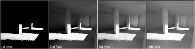
Radiosity is usually the algorithm for calculating those values. Basically it divides the scene into many small patches and generates form factors between each two patches and then makes some interations. During the first iteration, only emissive patches have energy, they distribute those energy to other visible patches. After the first iteration, patches directly visible to emissive patches receive some energy, however there won’t be effects like color bleeding or multiple light bounces. Some patches will be totally black. With the second iteration, there are more patches with energy that can be distributed to other patches. Even if patches not directly visible to emissive patches, usually light sources, will be lit this time. After several rounds of iteration, it will reach equilibrium. It should give a good result. Check here for more detailed explanation.

The algorithm is not suitable for non-lambertian brdf surfaces. For example, mirrors will not be rendered correctly with this technique alone because the lambertian brdf is totally different from a highly reflective brdf. And it is extremely slow.

Light Map Limitation

The robustness of an algorithm depends on the assumption it makes. Since we are focusing on static objects and static lights, those two are sort of acceptable. You can totally add dynamic light contribution during rendering. However not all of the surfaces are lambertian in the real case. Some have mirror like appearance, which will cause caustic and that’s why there won’t be caustic in light map. Anyway, those are not serious limitation.

One big advantage of light map over dynamic light computation during rendering is that there will be multiple light bounces, like color bleeding and soft shadow, although they are all static most of the time. So it usually represents low-frequency information, which is another implicit assumption made by light map algorithm. With this assumption, resolution of light map can be substantially reduced. We don’t usually allocate large memory for light map so that there is a one on one correspondence between texels in light map and texels in diffuse map. Light map usually needs to cover the whole scene. Although diffuse map also needs to cover the whole scene, it is usually tiled or repeated when sampled. It won’t be the same for light map, it is usually not tiled. The issue is if there is no one on one relationship between texels, there is no way to bake detailed information like variations caused by normal map. That’s why the scene looks flat with only light map.

In order to show variance brought by normal map, directional light map is introduced to solve the issue.

Directional Light Map

The reason we don’t have normal map variance when rendering with light map is that the irradiance value collected during pre-processing is integrated over the hemisphere around the geometry normal, not the surface normal defined through normal map or other method. It is valid to use the surface normal during preprocessing, however it will ends up in the issue of large light map memory that we tried to avoid in the first place.

Another impractical solution is to generate irradiance environment map at every position sampled in the scene. During rendering, the irradiance value could be retrieved through irradiance environment map and the surface normal. Regardless of the memory usage, it is the ideal solution for the issue. An advantage over the solution mentioned above is that it will support for dynamic normal because irradiance value is available for every direction. However the huge memory requirement renders it totally useless.

Spherical Harmonics

One practical solution for directional light map is using spherical harmonics to represent the irradiance environment map. Usually a couple of float numbers are needed to store the irradiance environment map and it is much more practical comparing with storing irradiance map directly.

The disadvantage is that there is still a great amount of memory needs to be stored in light map and it takes some extra cost than a normal light map algorithm because it is necessary to reconstruct the irradiance value with spherical harmonics.

Radiosity Normal Map

A much more practical solution is proposed by Valve, it is called radiosity normal map by them. It is not physically correct, however it works pretty well in the real case.

Instead of integrating over the hemisphere around geometry normal, three different basis are used during baking irradiance. That gives three different irradiance value for each sampled position.

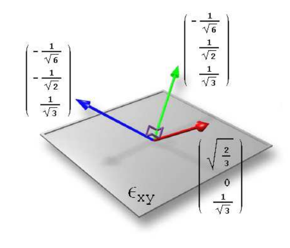
Those three basis are not arbitrarily chosen. They are pairwise orthogonal and cover the whole hemisphere. The reconstruction process is relatively simple:

$$ \begin{array} {lcl} color &=& dot( normal , basis[0] )^2 * lightmap\_color[0] + \\ & & dot( normal, basis[1] )^2 * lightmap\_color[1] + \\ & & dot( normal , basis[2] )^2 * lightmap\_color[2] \end{array} $$

Please note that the equation above is not exactly the same with the one mention in the paper by valve, it is the one from real time rendeing. Because the equation in the paper is incorrect. Since it is orthogonal basis that the normal projects on, there is no need to normalize the factors because the summation of the squared projected values is exactly 1.

Source engine by Valve uses this method. And Unreal Engine 3 uses a simpler version of it, only one irradiance value and three intensity value (three numbers) are stored. Instead of blending among the three, intensity values are blended and then multiply the irradiance value. So varying per-pixel values in normal map can only produce different brightnesses of the lightmap texel color instead of different colors.

If normal is not used for other purpose, normal map can be changed in another different form. Instead of storing normal in it, the squared projected values of the normal on the basis can be stored in it. And it can save many hardware cycles during real time calculation. Here is more detailed explanation.

Other methods

There are also other methods targeting on directional light map. Anyway, each of them tries to add more detail through their pre-baked light map and the basic rule always stands out, taking normal into account during light calculating of each frame rendering.

Conclusion

Directional light map is an extension to traditional light map algorithm, it takes surface normal intro account during rendering, which brings much more detailed information to the final generated image.

Although it may introduces a couple of extra instructions comparing with the old normal map, it is quite affordable even on mobile devices, that’s why UE3 has an internal implementation of it on mobile. Given the extra quality it brings, those cost should be considered worthy.

Reference

[1] Directional Light Map, Unity document
[2] Directional Lightmap
[3] Physically Based Rendering
[4] Real Time Rendering