Unit test for BXDF in offline rendering turns out to be way more important than what I thought it would be. I still remember it took me quite a long time when I debugged my bi-directional path tracing algorithm before I noticed there was a little BXDF bug, which easily led to some divergence between BDPT and path tracing. Life will be much easier if we could find any potential BXDF problem at the very beginning.

Unlike most simple real-time rendering applications, it requires a lot more than just evaluating a BXDF in pixel shader. Usually, in offline rendering, we need to support the following features for each BXDF:

• Evaluating BXDF given an incoming ray and out-going ray.
• Given a pdf and an incoming ray, we need to sample an out-going ray based on the pdf.
• Given an incoming ray and the same out-going ray generated above, it should return exactly the same PDF given by the above method. Keeping this consistent with the above feature is very important, otherwise, there will most likely be bias introduced in the renderer.
• It is usually hard-coded that which PDF we will use for a specific BXDF. Technically speaking, unlike the above features, one can totally ignore this one. The more similarities between the shape of the two functions, the faster it converges to the ideal result.

In this blog, I will talk about how PBRT verifies its BXDF in its ‘bsdftest’ program.

How the verification works

Following is one of the outputs from the verification program

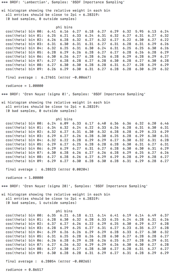
It is fairly clear that it shows results for three BRDFs. If we look at the output information closely, we will notice the following detail.

• We have a histogram with 10 x 10 entries in it. The whole sampling hemisphere domain is divided into 100 sub-domains, each of which has a same solid angle.
• Each of the entries should approach 2 * PI.
• The final average should also approach 2 * PI.
• There are two kinds of special samples
  • Bad samples. A sample with invalid data, like invalid radian or pdf.
  • Outside samples. Samples that are below the hemisphere.
• Evaluated radiance, which is really not important in this program.
• It may also output a warning if PDF evaluated based on the incoming and out-going ray doesn’t equal to the PDF we use to generate the out-going ray based on the incoming ray.

One can almost guess most of the things done in this application. Actually what this process does is this:

• First of all, it creates a sub-set of pbrt’s BXDFs, not the full set. That said it doesn’t verify every BXDF in the renderer. Since all of the BXDF in the applications are actually BRDF, it only considers samples in the upper hemisphere.
• For each BRDF, it takes 10000000 samples based on importance sampling provided by the BRDF. For each sample, it falls in a bad sample category if it has invalid data, it will be an outside sample if it is under the surface. Otherwise, based on the angle, it will be distributed to an entry in the histogram.
• Once the data in the histogram is generated, the output is generated by some mathematical formula. Basically, we need to pay attention to the error, bad/outside samples, or any invalid PDF error. A BXDF is considered OK if there are no bad samples, no PDF error and everything equals to 2 * PI. The number of outside samples is also important, but it is OK to have some, which means that the efficiency of this importance sampling may not be very good, but it is far from a sign of an existed bug in the renderer.

In the following sections, we will mainly talk about the mathematical formulas.

Why everything has to be 2*PI

Final average needs to converge to 2*PI

It is easier to explain why the final has to be 2*PI first, which is a pretty good start for this blog.

First of all, we can easily derive the following formula, which says that the area of a hemisphere where the radius is one is 2 * PI.

$$ \int_{\Omega} \mathrm{d}w = 2 * PI $$

Although we know it is 2 * PI, but let’s assume that we don’t so far. In order to evaluate $ \int_{\Omega} \mathrm{d}w $ , we can use Monte Carlo to solve it. The estimator is as follow:

$$ \dfrac{1}{N} \sum\limits_{i=1}^{N} \dfrac{1}{p({\omega}_i)} $$

If we look at the source code of this application, this is exactly what the verification does to calculate the final average. It is just a little bit less obvious because it accumulates the result in 100 bins first before calculating the final sum, but it is essentially the same math formula under the hood. In a nutshell, the final average is the estimator in this case.

Since we already know the value of the integral is 2 * PI. It means that the final average should converge to 2 * PI, with 10000000 samples taken, it could very likely indicate a bug if it doesn’t converge there.

About each entry

This one is a little bit more complex. But the basic idea is quite similar to the above derivation.

First of all, we need to pay attention to the way the algorithm divides the hemisphere domain. For phi, it is evenly divided into 10 equal-size region. For theta, it is very important to notice that it is the result of cosine theta that is evenly divided, not theta itself. So that said, theta is divided in the following sub-region.

$$ [acos(\dfrac{i}{10}), acos(\dfrac{i+1}{10})) $$

In the above formula, i goes from 0 to 9. For the last sub-region, it is fully inclusive. It may be very confused to see it is divided this way. But if we look at the solid angle extended by each sub-region, we will suddenly understand why it works this way.

$$ \begin{array} {lcl} \int_{{\Omega}_{ij}} \mathrm{d}{\omega}  & = & \int_{2*PI*i/10}^{2*PI*(i+1)/10} \int_{acos({(j+1)/10})}^{acos(j/10)} sin(\theta)\mathrm{d} \theta\mathrm{d} \phi \\\\ & = &\int_{2*PI*i/10}^{2*PI*(i+1)/10}\mathrm{d} \phi \int_{acos(j/10)}^{acos({(j+1)/10})}\mathrm{d}(cos(\theta)) \\\\ & = & 2*PI/100 \end{array} $$

The size of the solid angle is in-dependent of which sub-region it is casted from. The solid angle extended by the sub-region turns out to be same size!

Next, let’s define a visibility function so that we can focus on a single entry.

$$ V_{i j }(\omega) = \begin{cases} 1&:\theta \in [acos((i+1)/10),acos(i/10))  ,  \phi \in [2*PI*j/10,2*PI*(j+1)/10) \\ 0 &:otherwise \end{cases} $$

This visibility function gives you only the visibility of a single entry, leaving the rest of them as zero so that we can easily focus on one single entry. Since we divide the two-dimentional domain into sub-domain, i and j can identify which sub-domain we are focusing on. We can easily derive the following equation:

$$ \int_{\omega} V_{ij}(\omega) \mathrm{d}(\omega) = \int_{{\Omega}_{ij}} \mathrm{d}{\omega} = 2 * PI / 100 $$

Again, let’s look at the Monte Carlo estimator for the left-most integral in the above equation.

$$ \sum\limits_{k=1}^{N} \dfrac{V_{ij}(\omega)}{p(\omega_k)} $$

Basically, it says that if the sample falls in the subdomain defined by i and j, we count the contribution ( 1 / pdf ), otherwise we simply ignore it. N is the number of total samples taken, instead of just the samples falling in the subdomain. If we connect the two equations, we knows that by multiplying the result of the estimator by 100, we should reach 2 * PI. Which is exactly what the verification process does.

What does the process verify

Basically, it is most likely to expose a hidden bug in the bxdf implementation if there were something wrong with the following cases:

• A sampling process doesn’t generate samples based on given PDF at all.
• The pdf evaluation returns the incorrect value for an incoming and outgoing ray. Put it in another way, it doesn’t match the way we sample rays.

These are not something easy to find once there is bug. Locating the bug in bxdf during debugging a path tracing algorithm is way more painful than limiting the problem in a specific BXDF system.

Although it does verify something in bxdf, it doesn’t tell how good a PDF is to a bxdf. This is also something can be evaluated in a unit test.

References

[1] Physically Based Rendering, second edition