I read about this instant radiosity algorithm in the book physically based rendering 3rd these days. It is mentioned as instant global illumination though, they are actually the same thing. I thought it should be a good algorithm until I have implemented in renderer, I’m afraid that it is not quite an efficient one. Although it is also unbiased like path tracing and bidirectional path tracing, the convergence speed is just terribly low comparing with the others. It can barely show pure specular materials objects, it definitely needs special handling on delta bsdf. Since it is already implemented, I’ll put some notes on it.

Basic Idea

Instant Radiosity is pretty close to light tracing. Both of the algorithms trace rays from light sources instead of camera. The only difference between the two algorithm is where they connect vertices. In a light tracing algorithm, vertices along the light path are connected to camera directly. However in an instant radiosity algorithm, primary rays are still generated. Light path vertices are connected to the primary ray intersections then. The two algorithms are subset of bidirectional path tracing. Light tracing counts the path with only one vertex (eye vertex) in the eye path and instant radiosity only takes two-vertices length eye path into account.

The other big difference is that the light path is not for per-sample any more. With vertices in a number of light paths pre-calculated, all of the pixel samples use the same set of vertices instead of generating them during their radiance evaluation. I think that is where it differs most from other algorithms. In some senses, it can be explained this way, many virtual point light sources are distributed in the scene before evaluating each pixel value. After these virtual lights are well distributed, further evaluation of radiance can only consider ‘direct illumination’ w.r.t to both of real light sources and virtual light sources.

An interesting fact of this algorithm is that it converges to the correct result in a quite different way comparing with other algorithms, like path tracing. In a path tracer, if you have less number of samples, you usually get noisy results. While the results with less number of light paths in instant radiosity look more likely to be smoothly illuminated with a couple of light sources, just matches the above explanation. See the following images generated with roughly same amount of time by instant radiosity and path tracing, the left one calculated by instant radiosity gets quite smoother shading, while the right one is pretty noisy. I can’t say smoother is better, we definitely have some noticeable artifacts on the left result. First, the virtual shadows easily catch our attention even if there is only one real point light in the cornell box. Second, it is totally black on this right mirror like box. Third, we have some hotspot around the corner inside this cornell box.

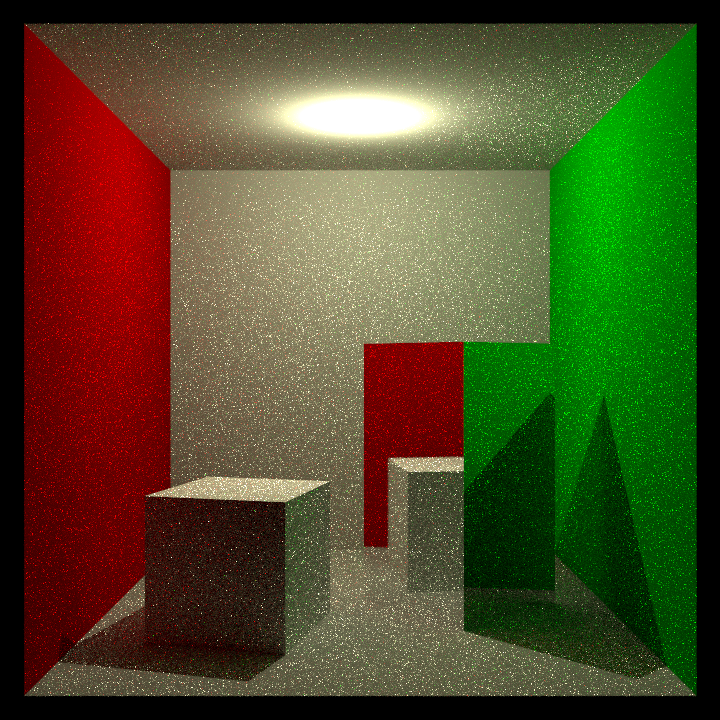
Of course, that is not to say it is a biased algorithm, it is just because we have only limited number of light paths generated in preprocess stage. With more light paths generated, those artifacts should be gone eventually. However, only the first issue can be hidden in a reasonable speed. The second issue usually needs explicit handling, like the way we handle it in a whitted ray tracer. We’ll talk about how to handle the last one later.

Math Behind It

The math behind it is much less complex than MIS bidirectional path tracer mentioned on my previous post. And since it is necessary to trace primary rays too, we don’t need to consider primary ray pdf because it is cancelled with importance function. It leaves us really simple mathematics behind the algorithm. We just need to evaluate the following equation correctly:

$$ L(p,w_i) = {\int...\int} \prod_{i=1}^{k-1}(f_r(x_{i+1} \rightarrow x_i \rightarrow x_{i-1} )G(x_i\longleftrightarrow x_{i+1})) L_e(x_k\rightarrow x_{k-1}) d(x_2) d(x_3) ... d(x_k) $$

This is not the whole rendering equation, it just stands for radiance value contributed by k+1 vertices length path, including both camera vertex and light vertex. For an unbiased renderer, it needs to evaluate the above equation for every possible k value, where k usually starts from 2 in the case of direct visible light. For a Monte Carlo estimator, it uses the following equation to approach the integral:

$$ L(p,w_i) = \dfrac{1}{N}\Sigma_{i=1}^N(\dfrac{\prod_{i=1}^{k-1}(f_r(x_{i+1}\rightarrow x_i\rightarrow x_{i-1})G(x_i\longleftrightarrow x_{i+1}))L_e(x_k\rightarrow x_{k-1})}{\prod_{i=2}^{k} p_a(x_i)}) $$

Since there are two stages in this algorithm, we can only evaluate part of the equation in the first stage, it is the part that doesn’t involve the x1 and x0, they should be two bsdf evaluation and a gterm.

$$ \begin{array} {lcl} L(p,w_i) &=& \dfrac{1}{N}\Sigma_{i=1}^N(\underbrace{f_r(x_2\rightarrow x_1 \rightarrow x_0)G(x_1\longleftrightarrow x_2)f_r(x_3\rightarrow x_2 \rightarrow x_1)}_{sample\, radiance\, evaluation\, in\, stage2} \\\\ &=& \prod_{i=3}^{k-1}(\underbrace{\dfrac{f_r(x_{i+1}\rightarrow x_i\rightarrow x_{i-1})G(x_i\longleftrightarrow x_{i-1})}{p_a(x_{i-1})}}_{stored\,in\,vertex\, during\, light\, path\, tracing\, in\, stage1})\dfrac{G(x_k\longleftrightarrow x_{k-1})L_e(x_k\rightarrow x_{k-1})}{p_a(x_{k-1})p_a(x_k)}) \end{array} $$

Although it may look more complex by a first look, however it is actually more clear for implementing the algorithm. As we can see from the above equation, the first two brdf and g-term are to be evaluated in radiance sampling in the second stage. While the rest of the equation should be done in the pre-process stage 1, which distributes virtual point lights around the whole scene. And it can be done in an incremental way, just like we trace rays in a path tracer. To be simpler, the above equation can be further simplified since we don’t actually pick samples w.r.t area, we sample new vertex by bsdf pdf w.r.t to the solid angle.

$$ \begin{array} {lcl} L(p,w_i) &=& \dfrac{1}{N}\Sigma_{i=1}^N(\underbrace{f_r(x_2\rightarrow x_1 \rightarrow x_0)G(x_1\longleftrightarrow x_2)f_r(x_3\rightarrow x_2 \rightarrow x_1)}_{sample\, radiance\, evaluation\, in\, stage2} \\\\ & & \prod_{i=3}^{k-1}(\underbrace{\dfrac{f_r(x_{i+1}\rightarrow x_i\rightarrow x_{i-1})cos\theta_{i\rightarrow i-1}}{p_w(x_i\rightarrow x_{i-1})}}_{stored\,in\,vertex\, during\, light\, path\, tracing\, in\, stage1})\dfrac{cos\theta_{k\rightarrow k-1}L_e(x_k\rightarrow x_{k-1})}{p_w(x_k \rightarrow x_{k-1})p_a(x_k)}) \end{array} $$

This is pretty clear for implementing the algorithm. After the first stage is done, we only need to trace one ray segment for evaluate each virtual point light’s contribution, no matter how long the path actually is.

Handling the Artifacts

As we can see from the above comparison, we can’t get anything from the mirror like box because it is almost delta function. In a practical ray tracer, it definitely needs special treatment for delta bsdf. Sadly, there is no delta bsdf support in my renderer, the mirror like material is actually a microfacet bsdf with 0 as roughness value. I’m not sure if there is a practical way to handle materials like this.

The other artifact that we can handle is those hot spots at the corner of the Cornell box. Those high lighted area is caused by connecting quite near vertices, resulting in a very large g-term value. According to the book, advanced global illumination, we can add a very small bias in the denominator of gterm to avoid those large values so that we can remove the hot spots by introducing bias into the method, which is unnoticeable. I can’t say that I agree with the idea, it is totally visible to me. Pbrt book introduces a great way of removing those ugly hot spot, it works pretty well to me. However I made a tiny change in the original method. My method is to clamp the inverse of the squared distance in the gterm when connecting vertices. Clamping it will definitely introduce a bias which is not something that I’d like to see, in order to get our unbiased feature back, we’ll add more code to handle it.

$$ \begin{array} {lcl} G(x_1,x_2) &=& \dfrac{cos\theta_{1\rightarrow 2} cos\theta_{2\rightarrow 1}}{|x_1 - x_2|} \\ &=& cos\theta_{1\rightarrow 2} cos\theta_{2\rightarrow 1} ( min( \dfrac{1}{|x_1-x_2|} , g_{clamp} ) + max( \dfrac{1}{|x_1-x_2|} - g_{clamp} , 0 ) ) \\ &=& \underbrace{cos\theta_{1\rightarrow 2} cos\theta_{2\rightarrow 1} min( \dfrac{1}{|x_1-x_2|} , g_{clamp} )}_{evaluate\, the\, same\, way} + \underbrace{cos\theta_{1\rightarrow 2} cos\theta_{2\rightarrow 1} max( \dfrac{1}{|x_1-x_2|} - g_{clamp} , 0 )}_{evaluate\, recursively} \end{array} $$ $$ G_0(x_1,x_2)=cos\theta_{1\rightarrow 2} cos\theta_{2\rightarrow 1} min(\dfrac{1}{|x_1-x_2|},g_{clamp}) $$ $$ G_1(x_1,x_2)=cos\theta_{1\rightarrow 2} cos\theta_{2\rightarrow 1} max(\dfrac{1}{|x_1-x_2|}-g_{clamp},0) $$ $$ G(x_1,x_2)=G_0(x_1,x_2)+G_1(x_1,x_2) $$

Now we’ve split the equation into two different parts and it equals to the original equation. We can them divide the extended rendering equation into two respectively.

$$ L(p,w_i) = L_0(p,w_i) + L_1(p,w_i) $$ $$ L_0(p,w_i) = {\int...\int} G_0(x_1,x_2) f_r(x_2 \rightarrow x_1 \rightarrow x_0) \prod_{i=2}^{k-1}(f_r(x_{i+1} \rightarrow x_i \rightarrow x_{i-1} )G(x_i\longleftrightarrow x_{i+1})) L_e(x_k\rightarrow x_{k-1}) d(x_2) d(x_3) … d(x_k) $$ $$ L_1(p,w_i) = {\int...\int} G_1(x_1,x_2) f_r(x_2 \rightarrow x_1 \rightarrow x_0) \prod_{i=2}^{k-1}(f_r(x_{i+1} \rightarrow x_i \rightarrow x_{i-1} )G(x_i\longleftrightarrow x_{i+1})) L_e(x_k\rightarrow x_{k-1}) d(x_2) d(x_3) ... d(x_k) $$

The first part clamps the value to a maximum limit in order to avoid high radiance value by connecting two near vertices. Really simple, there is nothing to say about it.

The second part is where the trick is. It would make no difference if we evaluate the equation the same way, because there is no upper limit on the inverse squared distance term. Instead of connecting the primary ray intersection with light path vertices, we sample a new ray based on the bsdf pdf, exactly like the way we do in a path tracer and then evaluate the radiance value recursively so that we can skip the super near vertex connection. Here is the math proof why it eliminates the near connection, only relative parts are shown:

$$ max( \dfrac{1}{|x_1-x_2|} - g_{clamp} , 0 ) dA(x_2) = max( 1 - \dfrac{g_{clamp} | x_2 - x_1 |}{cos\theta_{1 \rightarrow 2}}) dW(x_2) $$

The squared distance switches from denominator to the numerator, that’s why we won’t be affected by short distance vertices connection. A detail here is that during the recursive radiance evaluation, we treat the secondary ray as fake primary ray and the virtual light source which is very near to it won’t connect to it again because virtual light sources don’t affect directly illumination in the algorithm. A interesting fact here is that if g_clamp is 0, it switches from instant radiosity to path tracing.

Limitation of the Algorithm

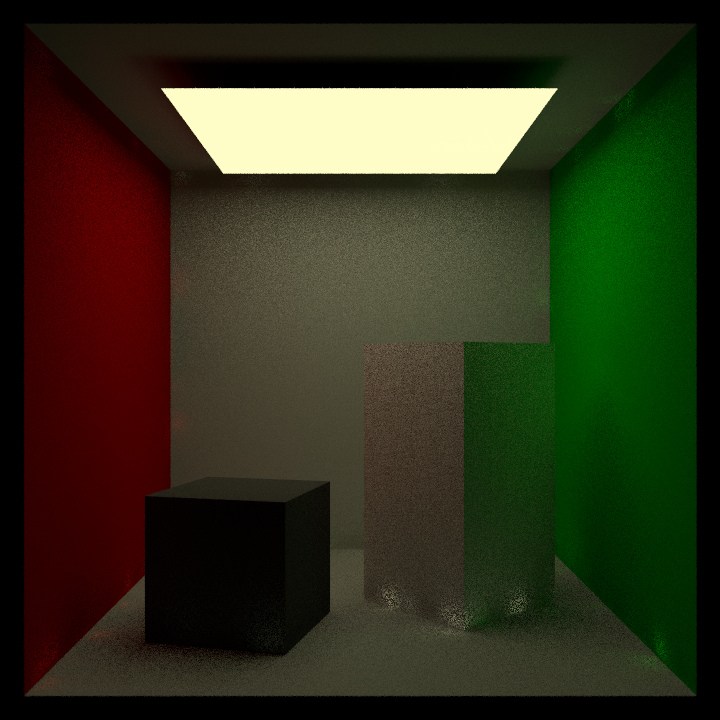
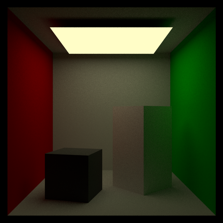
To tell the truth, I can’t justify many reasons to use the algorithm comparing with others, it converges quite slowly for mirror like materials and shows high light at corners. Even with the above trick, it is still hard to get similar result with other methods with only limited number of light paths, by limited number of light paths, I am talking about thousands. I tried 1024 light paths generated in the preprocess, it still can’t eliminate those artifacts. See the below images, left result is from instant radiosity, right one uses MIS bidirectional path tracing. The first one uses almost double time than the bdpt result. And that already gives me enough reason to switch to other more robuse algorithms like path tracing, bidirectional path tracing.

Reference

[1] Physically Based Rendering, 3rd
[2] Advanced Global Illumination
[3] Instant Radiosity