The book physically based rendering doesn’t spend too much effort explaining MIS, however it does mention it. In order to be more familiar with MIS(Multiple Importance Sampling), I spent some time reading Veach’s thesis. The whole thesis is relatively long, however the chapter about MIS is kind of independent to the other ones. Worth taking some notes in case I forget later.

Monte Carlo Integral

Monte Carlo tries to solve integral problem by random sampling. Basically it takes N independent samples randomly across the whole domain and use these samples to evaluate the integral.

$$ I = \int_{\Omega} f(x) \, \mathrm{d}x $$

Assuming here is the integral to be evaluated. Monte Carlo method is quite simple. First, N independent samples $ x_0,x_1, ... x_n $ are generated according to some property density function p(x). Then the estimator is like this:

$$ F_{N} = \dfrac{1}{N} \sum\limits_{i=1}^{N} \dfrac{f(x_i)}{p(x_i)} $$

The estimator is unbiased. In other words, the average of the estimator is exactly the integral we target on.

$$ \begin{array} {lcl} E[F_{N}] & = & E[\dfrac{1}{N} \sum\limits_{i=1}^{N} \dfrac{f(x_i)}{p(x_i)}] \\\\ & = & \dfrac{1}{N}\sum\limits_{i=1}^{N}\int_{\Omega} \dfrac{f(x_i)}{p(x_i)} p(x_i) d(x) \\\\ & = &\int_{\Omega} f(x) \, \mathrm{d}x \\\\ & = & I \end{array} $$

Just having the average value equaling to the integral doesn’t solve the problem, it is necessary to make sure that it converge to the right one as the number of samples grows. The variance approaches to zero if N keeps growing.

$$ \begin{array} {lcl} V[F_{N}] & = & V[\dfrac{1}{N} \sum\limits_{i=1}^{N} \dfrac{f(x_i)}{p(x_i)}] \\\\ & = & \dfrac{1}{N^2}\sum\limits_{i=1}^{N} V[\dfrac{f(x_i)}{p(x_i)}] \\\\ & = &\dfrac{1}{N}V[\dfrac{f(x)}{p(x)}] \\\\ & = & \dfrac{1}{N}( \int_{\Omega} \dfrac{f^2(x)}{p(i)} d(x) - I ) \end{array} $$

According to Chebychev’s inequality, we have:

$$ Pr\{|F_{N} - I|\ge\sqrt{\dfrac{V[\dfrac{f}{p}]}{N\delta}}\}\le\delta $$

That said the estimator convergences to the value of integral. It is consistent.

Combined with the two properties, the conclusion is that as long as we have enough samples, the result gets to the correct one we want to evaluate in the first place. And that is how we usually solve the integral problems in computer graphics.

There are several benefits with this method:

• Monte Carlo is general is relatively simple. Sampling according to specific pdf and evaluating the values at sampling positions are all that is needed to perform the calculation.
• Evaluating multi-dimensional integral is straightforward. Taking samples over the whole multi-dimensional domain is the only difference.
• It converges to correct value at a rate of $ O(N^{0.5})$ and the fact holds for integrals with any number of dimensions.
• Comparing with quadrature method, it is not sensitive to the smoothness of the function. Even if there is discontinuity at unknown position in the function, Monte Carlo can also deliver the same rate of convergence, which is $ O(N^{0.5})$ .

Consistent and Unbiased

There are two terms mentioned above, consistent and unbiased. Although they may look similar to each other at first glance, they are totally different concept.

The estimator is unbiased if:

$$ E[F_{N}-I] = 0 $$

An estimator is said to be consistent if it satisfy the following condition:

$$ \lim_{N\to\infty} P[|F_{N}-I|>\epsilon]= 0 $$

According to this wiki page, an unbiased estimator which converges to the integral value is said to be consistent. These two terms look quite similar to me, I actually thought one is the other’s super set. However it is not the case.

• $ F_{N}(X) = X_{1} $
  This one is an unbiased estimator, however it never converges to anything.
• $ F_{N}(X) = \dfrac{1}{N}\sum x_i + \dfrac{1}{N} $
  This is a consistent estimator, while it is biased.

My take here is that for unbiased estimator, as long as we compute the $ F_N$ multiple times and averaging the result will approach the right value. For consistent estimator, we need to increase the number of samples, which is N in this case, to achieve the right result. Photon mapping is a consistent method while it is not unbiased. It is consistent because you will approach the correct result by increasing the number of samples or photons. It is biased because you will never get something right by averaging the photon mapping result generated with just one sample, caustics won’t be sharp at all.

Importance Sampling

The first thing to do with Monte Carlo method is to pick a pdf first. Any pdf will give the right result, the simplest pdf for sampling is uniform sampling across the whole domain. Take a simple example here, to evaluate the following integral.

$$ I = \int_{0}^{1} f(x) dx $$

The Monte Carlo estimator is simply the average of all sampled values:

$$ F_N = \dfrac{1}{N} \sum\limits_{i=1}^{N} f(x_i) $$

However the problem is that the convergence rate may not be good if uniform sampling is used. Here is a further bad example from the book physically based rendering:

Here is the integral we want to evaluate:

$$ f(x)= \begin{cases} 0.01&:x\in [0,0.01) \\ 1.01&:x\in [0.01,1) \end{cases} $$

The integral value should be exactly one. Here is the pdf chosen for sampling:

$$ p(x)= \begin{cases} 99.01&:x\in [0,0.01) \\ 0.01&:x\in [0.01,1) \end{cases} $$

It is totally valid to solve the integral with Monte Carlo by this sampling. It will converge to the right value as the sample number increases, however the convergence speed is terrifically bad. Most of the samples taken will reside in the range of [0,0.01), which all give the estimated value of 0.0001(actually it is a little more than 0.0001). What is even worse is that when some are sampled in the range of [0.01,1), they give extremely high values, which is 101 in this case. On average, a huge number of samples are needed to get the right value. The variance of the sampling with this pdf is unnecessarily high.

On the other extreme, if the pdf is proportional to the integrated function, it gives you perfect correct result with just one sample. However it is never practical, because we won’t have certain knowledge about the function to be integrated most of the time. On the occasional cases where we know, we won’t bother to use Monte Carlo at all, because it may be integrated analytically.

The general idea of importance sampling is to evaluate the samples where they contribute more to the final result. The perfect case is the one mentioned above, however it is not practical most of the time. Even if the perfect pdf is difficult to find, finding a pdf with similar shape of the integrated function still provides great value because it will take samples where they contribute more. And that is called importance sampling, a practical way of reducing the variance without introducing too much overhead.

Here is the most common case in computer graphics, the function to be integrated is the rendering equation:

$$ {L_{o}(\omega_{o}) = \int L_{i}(\omega_{i}) *f( \omega_{i}, \omega_{o} ) *cos(\theta_{i}) d\omega_{i}} $$

Emission is dropped here for simplicity. The difficulty of evaluating this integral comes from certain aspects:

• Integrated function is a product of three different components, brdf, incoming radiance and cos factor.
• Although we can take samples according to cos factor and we may be able to take samples according to brdf, there is no way to have any knowledge about the incoming radiance for even slightly complex scene.

A typical way of solving this integral with Monte Carlo is to simply drop some factors with the hope that the dominate factors are not them. For example, by taking samples with the pdf proportional to the cos factor, it works pretty good for lambertain materials most of the time.

Multiple Importance Sampling

Importance sampling increases the convergence rate, however it is not everything. Sometimes you may need to take sample with different pdfs according to the situation.

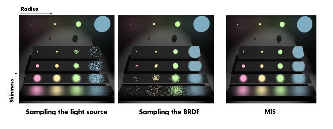
For example, for matte surfaces with small size light sources, it is better to sample the light source instead of the brdf. Because sampling the brdf will very likely miss the light and those samples that don’t miss the light will give relatively large result due to the small pdf value. On the contrary. for glossy surfaces with large area light sources, sampling the brdf will be better. Taking samples on the light source will probably contribute nothing to the final image and it really depends on how spiky the brdf is. The more spiky the brdf is, the better sampling brdf is. Below is an image of this situation. On the left it takes samples on the light source, there is clearly very low convergence rate for the top-right reflection. In the middle, it takes samples according to the brdf, for the lambertain surfaces, it works pretty badly with small light source. The right one is the result generated with MIS, we’ll get back later.

In general, the rule of thumb is to generate samples according to the pdf that is proportional to the dominant factor in the rendering equation. Although we might be able to switch between sampling brdf and sampling light source for the above case depending on the surfaces and light sources, most of the time we don’t even know which one of the three is the dominant one and that is the problem.

Instead of seeking to pick a perfect pdf for sampling, MIS goes another way by blending the results generated with different pdfs together without introducing noticeable noise.

Suppose $ n_i $ samples are taken for $ p_i(x) $ among n pdfs. The MIS estimator is simply:

$$ F_{mis} = \sum\limits_{i=1}^n \dfrac{1}{n_i} \sum\limits_{j=1}^{n_i} w_i(X_{i,j})\dfrac{f(X_{i,j})}{p_i(X_{i,j})}$$

For MIS estimator, the following conditions need to hold true:

• $ \sum\limits_{i=1}^{n}w_i(x) = 1 $ if $ f(x) \neq 0 $
• $ w_i(x) = 0 $ if $ p_i(x) = 0$

The MIS estimator is an unbiased one if the above conditions are fulfilled. Here is the proof:

$$ \begin{array} {lcl} E[F_{mis}] & = & E[ \sum\limits_{i=1}^n \dfrac{1}{n_i} \sum\limits_{j=1}^{n_i} w_i(X_{i,j})\dfrac{f(X_{i,j})}{p_i(X_{i,j})}] \\\\ & = & \int \sum\limits_{i=1}^n \dfrac{1}{n_i} \sum\limits_{j=1}^{n_i} w_i(x)\dfrac{f(x)}{p_i(x)} p_i(x) dx \\\\ & = & \int \sum\limits_{i=1}^n \dfrac{1}{n_i} \sum\limits_{j=1}^{n_i} w_i(x) f(x) dx \\\\ & = & \int \sum\limits_{i=1}^n w_i(x) f(x) dx \\\\ & = & \int f(x) dx \end{array} $$

Actually the Monte Carlo estimator can be seen as a specialized MIS estimator where one sample is taken according to a pdf and all pdfs are exactly the same, N samples are taken in total. Being written this way will make it more clear:

$$ F_{mis} = \sum\limits_{i=1}^N \dfrac{1}{1} \sum\limits_{j=1}^{1} w_i(X_{i,j})\dfrac{f(X_{i,j})}{p_i(X_{i,j})}$$

where all $ p_i(x) = p(x)$ and all $ w_i(x) = \dfrac{1}{N} $ . As a specialized MIS estimator, it has one issue that is the variance is additive and it misses the purpose we want to achieve in the first place.

Another special case of MIS estimator is to divide the whole domain into several and take samples in those domain separately. That is basically the method mentioned above, switching between brdf and light source depending on the environment. However it is not practical due to its simplicity. Sometimes you don’t know which one to sample.

Balance Heuristic

Finding good weight functions is crucial to the algorithm itself. The balance heuristic is a good one to start with.

$$ w_i(x) = \dfrac{n_i p_i(x)}{\sum\limits_{k}n_kp_k(x)} $$

By putting it into the MIS estimator, we have the following equation:

$$ F_{mis} = \sum\limits_{i=1}^n \sum\limits_{j=1}^{n_i} \dfrac{f(X_{i,j})}{\sum\limits_{k}^{n}n_kp_k(x)}$$

The variance will be reduced with this estimator. I don’t know the accurate proof of it. However from the equation, the estimator will be good as long as one of the pdf is similar to the function to be integrated. For example, let’s take a two pdf MIS case here:

$$ F_{mis} = \dfrac{f(X_{0,0})}{p_0(X_{0,0})+p_1(X_{0,0})} + \dfrac{f(X_{1,0})}{p_0(X_{1,0})+p_1(X_{1,0})} $$

Assume the first pdf is a good match for the function, at places where the value of this function is high, the first pdf will likely to take samples there and even if the second one is very small, the result won’t change much unless it is very high which will dimmer the result. However if the second pdf is extremely spiky, values of pdf across the domain outside this spiky area will be quite small and that affects little to the final result with MIS. Of course the domain with high pdf values will be affected for sure, the result there will be smaller. So pdf with extremely spiky shape should be avoided unless the function itself to be integrated is one.

Although MIS can reduce variance a lot, that doesn’t mean it is free to pick any pdf. Poor picking of pdf will result worse even if with MIS, like the one mentioned above. In general as long as the shape of pdf is similar to that of integrated function across part of the domain, it is a good one. The right most image above is the one generated with balance heuristic MIS.

Other Heuristics

There are also other heuristics available. The general idea of the other heuristics is to sharpen the shape of the weighting function, making values near 1 larger and values near 0 smaller.

The power heuristic:

$$ w_i = \dfrac{q_i^{\beta}}{\sum\limits_{k}q_k^{\beta}} $$

$ \beta $ i s 2 in pbrt implementation.

The cutoff heuristic:

$$ w_i= \begin{cases} 0&:q_i<\alpha q_{max} \\\\ \dfrac{q_i}{\sum\limits_{k}{\{q_k|q_k\ge\alpha q_{max}\}}}&:otherwise \end{cases} $$

$ q_{max} $ is the maximum one among all $ q_i$s .

The maximum heuristic:

$$ w_i= \begin{cases} 1&:q_i=q_{max} \\ 0&:otherwise \end{cases} $$

Conclusion

Monte Carlo method is a powerful tool solving the integrals in computer graphics. With importance sampling, the variance can be reduced a lot. And MIS makes it even practical by merging samples taken from different pdfs. Although it is not a perfect solution without any addition to the variance, it works pretty well in general.

References

[1] Physically Based Rendering, second edition
[2] Bias in Rendering
[3] Robust Monte Carlo Method for Light Transport Simulation