I’m working on microfacet brdf model for my renderer these days, noticing that it is more than necessary to provide a separate sampling method for microfacet brdf instead of using the default one, which is usually used for diffuse like surfaces and highly inefficient for brdf with spiky shape, such as mirror like surfaces. The following image is one generated by the default sampling method:

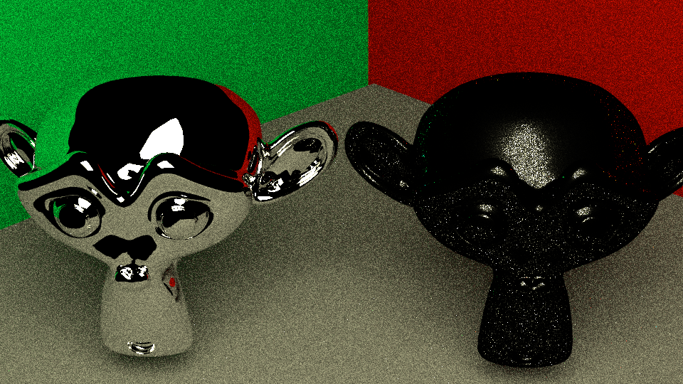
The left monkey has pure reflection brdf which is mentioned in my previous blog post, the right one uses the microfacet model with zero as roughness value. I was expecting similar result for both of the monkeys while things turned out to be wrong here, we can barely see the reflection from the monkey. Actually there is nothing wrong, the fact is that the convergence rate of default sampling the microfacet model with 0 roughness is extremely low. As long as there are enough samples, it will reach the appearance similar to the left one. However the number of samples being enough can be arbitrarily high depending on how spiky your brdf is.

The right way of sampling microfacet brdf is mentioned in this paper. What I want to write down in this blog is how these conclusions are derived from the original microfacet model. Using these better sampling methods, we will get similar result for those two monkeys eventually.

Why Default Sampling Method is Inefficient

So why is this default sampling method inefficient for mirror like brdf model. First of all, the default sampling method goes with the following pdf:

$$ p_h(\omega) = \dfrac{cos(\theta)}{\pi} $$

It achieves good result for diffuse surfaces like Lambert, OrenNayar. In fact, it is not a sampling method for diffuse brdfs, a sampling method for lambert brdf will respect a pdf with constant value, it also involves the cosine factor located in the rendering equation or LTE.

$$ {L_{o}(\omega_{o}) = \int L_{i}(\omega_{i}) *f( \omega_{i}, \omega_{o} ) *cos(\theta_{i}) d\omega_{i}} $$

Since it is extreme difficult, if not impossible, to have any knowledge on the incident radiance, the only thing we have is the brdf and cosine factor. The sampling method mentioned above could be efficient if the product of brdf and cosine factor is the dominant one in this equation. It works pretty well in practice most of the time.

However the efficiency of default sampling method tanks quickly as the brdf becomes the dominant factor with roughness going to zero. For microfacet brdf here, its extreme form is like a dirac-delta function, it is almost impossible to get a sample with brdf having a non-zero value. And for the lucky ones that do have non-zero brdf values, it could reach super high value due to its low probability, introducing high variance to the sampling result. In other words, the convergence rate is quite low, which is exactly why we are seeing the above image. It can be even treated as a bug. Obviously, we need a better way to sample these microfacet brdfs.

Microfacet Model

Microfacet Model is quite hot in real time rendering these years, it is the basics of physically based shading algorithm. Basically, its basic form is like the following:

$$ f(\omega_i,\omega_o,x) = \dfrac{F(\omega_i , h) G(\omega_i,\omega_o,h) D(h)}{4 cos(\theta_i) cos(\theta_o)}$$

The first component is Fresnel, the second one is a shadowing factor called G term, the last one is normal distribution function (NDF). Comparing with the old ad-hoc bxdf model, microfacet model obeys the rule of energy conservation which allows the artist to change the roughness of the material through one parameter instead of two, specular color and specular power.

Among all those factors in this equation, the NDF term is usually the dominant one. The specific shape of NDF is largely affected by the roughness of the bxdf. In order to sample the microfacet brdf model, it is usually to sample NDF first getting a random microfacet normal that respects the NDF and then reflect the exitence radiance along the normal to generate the incident direction.

There are several kinds of NDF around. The following three will be covered in this blog and all that will be mentioned are isotropic ones.

• GGX
• Beckmann
• Blinn

Before we proceed, there is one rule that all NDF should follow:

$$ \int_{\Omega} D(m) cos(\theta_m) d\omega = 1$$

We will use this equation in our following derivation. Explaining the equation is outside the scope of this blog, however one can refer here for further detail.

Sampling GGX

Here is the basic form of GGX:

$$ D(h) = \dfrac{\alpha^2}{\pi ((\alpha^2-1) cos^2\theta + 1 ) ^2} $$

So the pdf respecting solid angle is like this:

$$ p_h(\omega)=\dfrac{\alpha^2cos\theta}{\pi((\alpha^2-1) cos^2\theta+1)^2}$$

Instead of sampling solid angle directly, we usually use spherical coordinate to sample it. So it is not the pdf respecting the solid angle that we are interested, it is the pdf respecting the spherical coordinates.

$$ p_h(\theta,\phi)=\dfrac{\alpha^2cos\theta sin\theta}{\pi((\alpha^2-1) cos^2\theta+1)^2}$$

The following task is quite straight forward, which is basically sampling according to a specific pdf. Inversion method goes pretty well for all NDFs in this blog. Notice that $ \phi $ is not even in this equation, that said the NDF is totally isotropic and we can sample $ \phi $ uniformly. For detail proof, please refer here. The only thing left here is how to sample $ \theta $. In order to do that, we need to get the pdf for $ \theta $ first.

$$ p_h(\theta)=\int_{0}^{2\pi}p_h(\theta,\phi)d\phi = \dfrac{2\alpha^2cos\theta sin\theta}{((\alpha^2-1) cos^2\theta+1)^2} $$

Let’s calculate the CDF next:

$$ \begin{array} {lcl} P_h(\theta) & = & \int_{0}^{\theta} \dfrac{2\alpha^2 cos(t) sin(t)}{(cos^2t(\alpha^2-1)+1)^2}dt \\\\ & = & \int_{\theta}^{0} \dfrac{\alpha^2}{(cos^2t(\alpha^2-1)+1)^2}d(cos^2t) \\\\ & = & \dfrac{\alpha^2}{\alpha^2-1} \int_{0}^{\theta} d{\dfrac{1}{cos^2t(\alpha^2-1)+1}} \\\\ & = & \dfrac{\alpha^2}{\alpha^2-1} {(\dfrac{1}{cos^2\theta(\alpha^2-1)+1}-\dfrac{1}{\alpha^2})} \\\\ & = & \dfrac{\alpha^2}{cos^2\theta(\alpha^2-1)^2+(\alpha^2-1)}-\dfrac{1}{\alpha^2-1} \end{array} $$

With a random number ranging from 0 to 1 $ \epsilon $ that is equal to this CDF, we have the following equation:

$$ \epsilon =\dfrac{\alpha^2}{cos^2\theta(\alpha^2-1)^2 + (\alpha^2-1)} - \dfrac{1}{\alpha^2-1}$$

To solve this equation requires no more knowledge than mathematic in junior high school, I guess there is no need to show the whole process. The final solution of the above equation is:

$ \theta =arccos\sqrt{\dfrac{1-\epsilon}{\epsilon(\alpha^2-1)+1}} $ or $ \theta =arctan(\alpha\sqrt{\dfrac{\epsilon}{1-\epsilon}}) $

The above two equations are exactly the same thing. Choosing which one to use is just a matter of taste.

Sampling Beckmann

The derivation of sampling method for Beckmann is quite similar to the above procedure. Here is the Beckmann distribution:

$$ D(h) =\frac{1}{\pi\alpha^2cos^4\theta}e^{-\frac{tan^2\theta}{\alpha^2}}$$

The pdf respecting spherical coordinate is like this:

$$ p_h(\theta,\phi)=\frac{sin\theta}{\pi\alpha^2cos^3\theta}e^{-\frac{tan^2\theta}{\alpha^2}}$$

Again, $ \phi $ can be sampled uniformly. The pdf for $ \theta $ should be this:

$$ p_h(\theta)=\frac{2sin\theta}{\alpha^2cos^3\theta}e^{-\frac{tan^2\theta}{\alpha^2}}$$

The CDF for $ \theta $ can be calculated this way:

$$ \begin{array} {lcl} P_h(\theta) & = & \int_{0}^{\theta} \frac{2sin(t)}{\alpha^2cos^3t}e^{-\frac{tan^2t}{\alpha^2}}dt \\\\ & = & \int_{0}^{\theta} \frac{-2}{\alpha^2cos^3t}e^{-\frac{tan^2t}{\alpha^2}}d(cos(t)) \\\\ & = &\int_{0}^{\theta} \frac{1}{\alpha^2}e^{-\frac{tan^2t}{\alpha^2}}d(\frac{1}{cos^2(t)}) \\\\ & = & \int_{0}^{\theta} \frac{1}{\alpha^2}e^{\frac{1}{\alpha^2}(1-\frac{1}{\cos^2t})}d(\frac{1}{cos^2(t)}) \\\\ & = & \int_{\theta}^{0} d(e^{\frac{1}{\alpha^2}(1-\frac{1}{\cos^2t})}) \\\\ & = & 1- e^{\frac{1}{\alpha^2}(1-\frac{1}{\cos^2\theta})} \end{array} $$

Solving the equation of $ P_h(\theta) = \epsilon $ gives the following solution:

$ \theta =arccos\sqrt{\dfrac{1}{1-\alpha^2 ln(1-\epsilon)}} $ or $ \theta =arctan\sqrt{-\alpha^2\ln(1-\epsilon)} $

Sampling Blinn

Here is the Blinn NDF:

$$ D(h)=\dfrac{\alpha+2}{2\pi}(cos\theta)^\alpha$$

The pdf respecting to spherical coordinate is:

$$ p_h(\theta,\phi)=\dfrac{\alpha+2}{2\pi}(cos\theta)^{\alpha+1}sin\theta $$

Isolating $ \phi $ gives the following:

$$ p_h(\theta) = (\alpha+2)(cos\theta)^{\alpha+1}sin\theta $$

This one is a lot simpler than the previous two, here is the CDF:

$$ \begin{array} {lcl} P_h(\theta) & = & \int_{0}^{\theta} (\alpha+2)cos(t)^{\alpha+1}sin(t)d(t) \\\\ & = & \int_{\theta}^{0} (\alpha+2)cos(t)^{\alpha+1}d(cos(t)) \\\\ & = &\int_{\theta}^{0} d(cos(t)^{\alpha+2}) \\\\ & = &{1-cos(\theta)^{\alpha+2}} \end{array} $$

Here is the relation between random number and $ \theta $

$$ \theta=arccos((1-\epsilon)^{\frac{1}{\alpha+2}})$$

Since $ \epsilon $ is a uniformly distributed random number between 0 and 1, $ 1-\epsilon $ is the same. So we can simplify the above equation with the following one:

$$ \theta=arccos(\epsilon^{\frac{1}{\alpha+2}})$$

A little more about this sampling method. I’m not quite confident with this solution, although I can see nothing wrong in this derivation. PBRT gives a similar solution for Blinn which is:

$$ \theta=arccos(\epsilon^{\frac{1}{\alpha+1}})$$

And another open-source ray tracer, mitsuba, also adopts this way of sampling. I don’t quite understand the derivation in the book, so I’ll just stick to this one, which is also the one mentioned here. I tried the pbrt’s way of sampling, only minor difference can be noticed from the image.

One Extra Step

There is still one step further from being done. It is the incident direction sampling that we are interested, not the normal. The reason we are sampling the normal instead of incident direction directly is because NDF is usually the dominant factor in microfacet model. Generating the incident direction after sampling normal is a more efficient way than sampling the incident direction itself.

However the way we calculate PDF given an incident direction is different from the above ones respecting half-vector, whether it’s solid angle or spherical coordinate. What we have so far is the pdf for half-vector, a transformation is necessary.

$$ p(\theta) = p_h(\theta) \dfrac{d\omega_h}{d\omega_i} = \dfrac{p_h(\theta)}{4 (\omega_o \cdot \omega_h)} $$

Conclusion

Here are the images generated after and before the new sampling method.

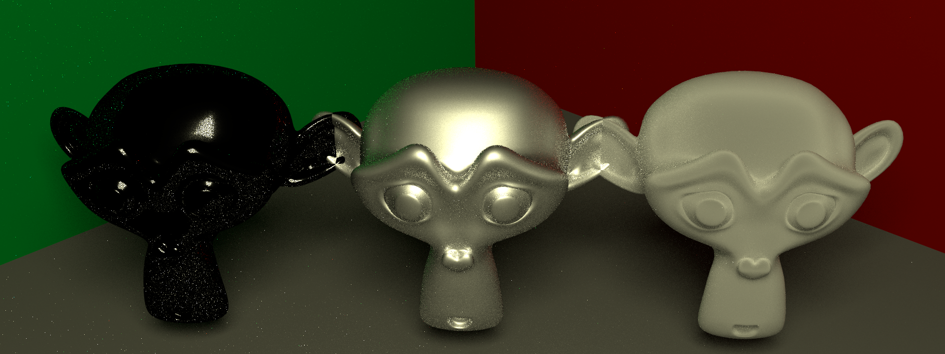
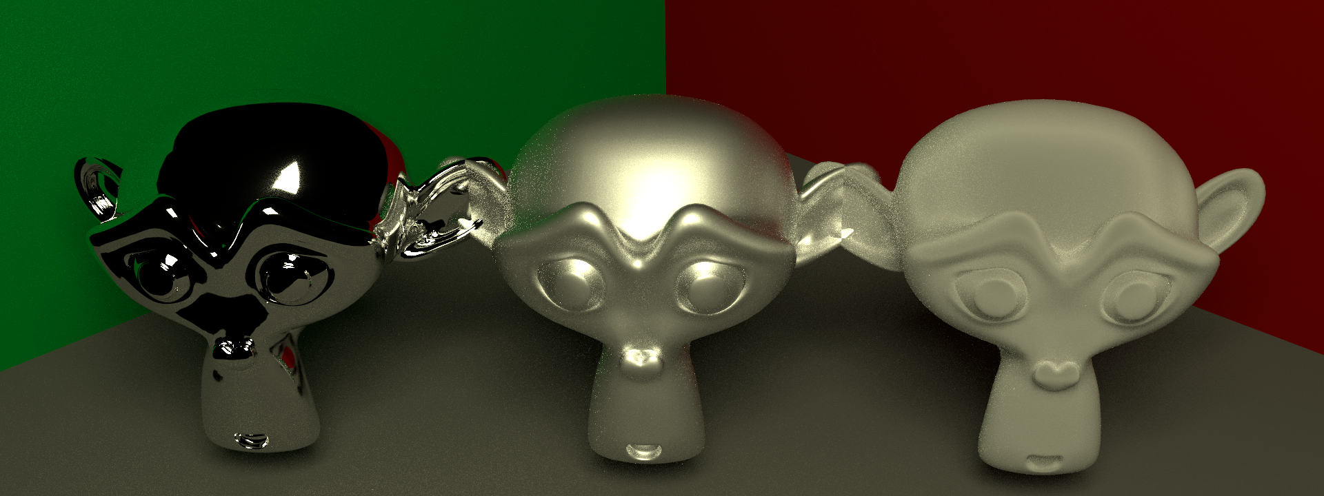
There are 64 samples per pixel and GGX is chosen as NDF, the three monkeys have different roughness values(0.0,0.5,1.0). As we can see from the image that the left-most monkey gets much better result than the default sampling method. And for the other two monkeys, we have similar result with the cosine-pdf sampling method.

There are already some research work improving the sampling method mentioned in this blog. I may need to try their method once I have some free cycles.

Reference:

[1] Microfacet Models for Refraction through Rough Surfaces
[2] Dirac delta function
[3] How is the NDF really defined
[4] Notes on importance sampling