Finally, I have some time reading books, spending several days digesting the volume rendering part of PBRT, there are loads of stuff that interest me. Instead of repeating the theory in it, I decided to put some key points in my blog with some brief introduction and then provide some derivations which are not mentioned in the book.

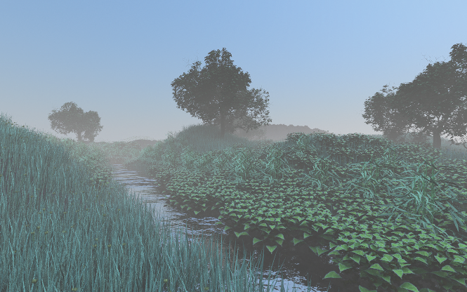
In case someone is not familiar with what volume rendering is, the above textures are attached for your references. One can easily notice that the fog on the right image greatly enhances the fidelity of the scene to a whole new different level. For a detailed explanation of volume rendering, it is suggested to check out this wiki page. Volume rendering is commonly used as fog, water etc. And mastering the basics behind it is of great importance because it also serves the basic theory of sub-surface scattering, which is very common even in real time 3D applications, like video games.

How Light Interacts with Volume

In a nutshell, volume can change the way light propagates, which is why we care. More specifically, volume consists tons of very small particles that can interact with light rays. Some of them change the direction of light rays, others will absorb some energy from the ray, some even emits energy. There are four types of interaction that we need to consider in an offline renderer:

• Absorption. Light will attenuate as it travels through a volume.
• Emission. Some volume may emit energy making itself a ’light source'.
• Scattering. There are two kinds of scattering:
  • Out-Scattering. This happens when the light ray changes its direction. This is why fog makes background dimmer.
  • In-Scattering. Since light can change its direction, there are chances that some light will come in due to light direction changing. A real case is why it appears grey in a foggy day, because fog bends the sun rays to your eye.

Real-Time Solution

Real-time solution for volume rendering is commonly biased. A quite common solution is particle system, meaning generating tons of billboards with alpha blending enabled. Most of the practical or research work aims at how to render a huge number of particles in an efficient manner. I haven’t seen any targeting on the unbiased feature of particle rendering, because it is not from the very beginning.

Of course, particle system can only deliver effects like smog, fire etc. It may not be able to reproduce some other volume like light shaft or water. Although a lot of water simulation work does use particles under the hood, we don’t usually call them particle system. Light shaft is commonly a post-processing pass, some work generate light shaft with real geometry, but I haven’t seen any work using particles to simulate it.

As hardware is getting more and more powerful. Modern AAA games also have lots of volume rendering in them, which is actually way out of the scope of this blog. For a short description and implementation, I strongly suggest walking through the implementation in this shadertoy demo.

Offline Solution

Comparing with real-time rendering solution, I kind of like offline solution due to its consistence among all situation like fog, light shaft or even water. I am no expert of physics, my take on them is that all of them are a set of particles at a micro level. They are actually the same except that the difference is how particles interact with each other.

Absorption

Let’s start from absorption. Assuming we have a volume with its particles uniformly distributed inside it, light attenuation due to absorption will be the same at all points along the ray.

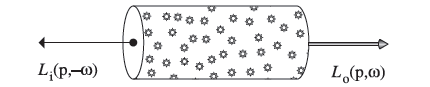
We have the following equation at a micro level:

$$ L_o(p,w) - L_i(p,-w) = dL_o(p,w) = -\sigma_a(p,w)L_i(p,-w)dt$$

This may look confusing the first time one sees it because of the subscripts, it adopts the commonly used term Li and Lo in it. Detail explanation is at the page of 286 of the book (second edition). After converting all subscript into one, we get the following equation:

$$ dL_o(p,w) = -\sigma_a(p,w)L_o(p,w)dt $$

And since the subscript is just something that we use to distinguish between incoming and outgoing light, we can drop it in the above equation making it much clearer than it used to be.

$$ dL(p,w) = -\sigma_a(p,w)L(p,w)dt $$

What it says is that light will attenuate with exactly the same rate at all points along the ray. Comparing with micro level equation, what we care more is a higher level knowledge of light interaction with volume, instead of small particles that are not visible to human vision at all. So the real practical question is how much light will still remain after passing through a uniform volume like the above one.

First of all, let’s convert the equation this way:

$$ \dfrac{dL(p,w)}{L(p,w)} = -\sigma_a(p,w)dt $$

One detail that we haven’t mentioned is the parameter of ’t’. Any point along the ray could be represented by $ p(t)=p(0) + t*w $. In other words, it is the distance between the starting point and ending point that we consider. So we can regard ‘p’ as a function of t in the above equation. If we take an integral from 0 to d, we have the following equation.

$$ \int_0^d \dfrac{dL(p(t),w)}{L(p(t),w)} = \int_0^d -\sigma_a(p(t),w)dt $$

It is quite easy to derive the following equation.

$$ \dfrac{L(p+d*w,w)}{L(p,w)} = e^{ -\int_0^d \sigma_a(p,w)dt} $$

The above equation is the attenuation, which only takes absorption into account, due to the existence of the volume. And it is exactly the second equation mentioned at the page of 578 in PBRT book (second edition).

Out-Scattering

Out-scattering is quite similar with absorption. As a matter of fact, there is no difference between them in handling attenuation. So instead of saving absorption factor, we can save attenuation factor which is the summation of absorption and out-scattering. Unless we have a clear reason to save them separately, there is no need to do that.

$$ \sigma_t=\sigma_a+\sigma_s$$

For our convenience, it is better to define one term, which is commonly named ‘beam transmittance’ and defines the proportion of light survives the uniform volume due to attenuation (out-scattering and absorption).

$$ T_r(p(0) \rightarrow p(d) ) = e^{ -\int_0^d \sigma_t(p,w)dt} $$

Emission

Emission is actually the simplest one among the four. The differential change is just the emission rate.

$$ dL(p,w) = L_{e}(p,w)dt $$

In-Scattering

This is the most complex one among the four, it took me a while to figure out the mathematics behind it. I’d like to start with two equations in PBRT(2nd) and explain the derivation between them. First equation is the differential changes along the ray direction due to in-scattering.

$$ \dfrac{dL_o(p,\omega)}{dt} = -\sigma_t(p,\omega) L_i(p,-\omega) + S( p,\omega) $$

At a first glance, it seems weird due to the fact that it involves both $ L_i $ and $ L_o $. As a matter of fact, we can easily convert it to uniform direction by switching $ L_i $ to $ L_o $.

$$ \dfrac{dL_o(p,\omega)}{dt} = -\sigma_t(p,\omega) L_o(p,\omega) + S( p,\omega) $$

One good feature about it is that since we only have $ L_o $, we can safely drop that subscript making the equation simpler. Although all functions in this equation are functions of both solid angle and position, which is further a function of t, the distance from the original point as mentioned above, it is also safe to drop the solid angle parameter because it doesn’t change in the equation at all. We can further simplify the equation to the following state:

$$ \dfrac{dL(p)}{dt} = -\sigma_t(p) L(p) + S( p ) $$

What it says is really simple, it states the fact that the differential change due to in-scattering along the ray is the amount of differential in-coming scattering radiance S(p) minus the attenuation by absorption and out-scattering. For the simplicity, I won’t include the definition of S here. One can always read PBRT(2nd) for further information.

The other equation in PBRT is the following one, which according to the book can be derived from the above one.

$$ L_i(p,\omega) = \int_0^{\infty} T_r(p' \rightarrow p) S(p', -\omega) dt $$

Again, let’s get rid of the subscript first.

$$ L(p,-\omega) = \int_0^{\infty} T_r(p' \rightarrow p) S(p', -\omega) dt $$

If you look at the picture below, you will find that this description is even better than the previous one, although both make perfect sense. What it says is that the radiance at point p along direction -w due to in-scattering is actually the accumulation of all in-scattering radiance at all points along direction -w attenuated by its corresponding beam transmittance.

In order to derive from the first equation to the second one, we need to handle one small issue. Notice that the first equation proceed along the direction w, while the second one goes just in the opposite way. I choose to invert the first equation in my derivation. It becomes this:

$$ \dfrac{dL(p,-\omega)}{d(-t)} = -\sigma_t(p,-\omega) L(p , -\omega ) + S( p , -\omega ) $$

One subtle difference between this equation and the original one is that the differential denominator is -t instead of t. This is by no means a typo. This is because we invert the direction of the ray along -w. If we take the negative sign out of the denominator, we get the following equation

$$ \dfrac{dL(p,-\omega)}{d(t)} = \sigma_t(p,-\omega) L(p , -\omega ) - S( p , -\omega ) $$

One can easily notice that this is quite standard first order linear differential equation. The solution is available as the following one:

$$ L(p(t)) = \dfrac{1}{e^{-\int \sigma (p)dt}}( -\int e^{- \int \sigma (p)dt} S(p) dt + C ) $$

I’ll skip the derivation of the solution in this blog, one can find further detail here. And please also notice that the subscript of $ \sigma $ and the $ \omega $ are also dropped because they don’t change in the equation, but please notice that the L(p) in the following equation means L(p,-w). To solve the equation, the first thing to do is to determine the constant factor C. We already know that $ L(p( \infty)) $ is zero, dropping it in the equation, we can get C.

$$ C = \int e^{\int \sigma (p)dt} S(p) dt |_\infty $$

Again, we get the following equation by dropping the value of C in it.

$$ \begin{array} {lcl} L(p(t)) & = & \dfrac{1}{e^{-\int \sigma (p)dt}} \int_t^{\infty} e^{- \int \sigma (p)dt'} S(p) dt' \\\\ & = & \int_t^{\infty} e^{- \int_{t}^{t'} \sigma (p)dt''} S(p) dt' \end{array} $$

What we want is actually L(p(0)), letting t equals to zero, will give you the following equation:

$$  L(p(0)) = \int_0^{\infty} e^{- \int_{0}^{t} \sigma (p)dt'} S(p) = \int_0^{\infty} T_r(p(t) \rightarrow p(0)) S(p(t)) dt $$

And with the above equation, we finished the derivation.

Reference

[1] Physically Based Rendering, second edition
[2] UCDavis, Mathematics. First order linear differential equation
[3] Volumetric Integration