Subsurface scattering has always been a challenge in computer graphics. Even in offline rendering, some of the common practical solutions are nowhere near unbiased. In certain algorithms, there are some pretty aggressive assumptions made to make things under control. However, despite the complexity in subsurface scattering algorithms, it is by no means a feature that can be missing from a practical rendering engine. Major commercial renderers, like Arnold, Cinema 4D, etc, all have very sophisticated and solid implementation of SSS. Robust implementation of SSS also exists in open-source projects, like Cycles and luxcorerenderer, and even some research-based projects maintained by only a handful of people, like PBRT and mitsuba. What is even amazing is that real-time rendering also has practical and efficient subsurface scattering implementation. In game industry, there is no shortage of amazing games with stunning and convincing skin rendering, for example, like the Last of Us Part II.

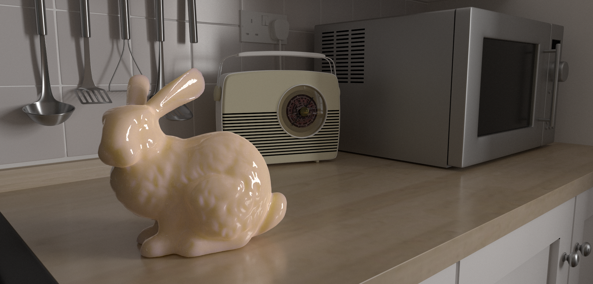
I happened to have some time last year and eventually finished an implementation that I’m satisfied with after quite a few iterations. Following is a shot using my renderer and it is a good example demonstrating the SSS feature in it. Also, all other images in this blog are rendered using my renderer too.

There are quite some resources about SSS theories on the internet. However, I rarely see any material revealing the specific details to be noted in implementing SSS algorithm. This could totally be because I haven’t done enough research work in this field. But it is still worth my time to put down all the notes I have during my iterations. Starting from integrating PBRT 3rd edition’s implementation, I quickly noticed that the implementation works for some cases, but there are cases where it fails to converge efficiently. By comparing with Cycles implementation, I made some progress with more iterations.

This blog is about the iterations that I have made on top of PBRT’s implementation. I will briefly mention the basics of SSS theory in PBRT. My introduction covers only part of what PBRT talks about in subsurface scattering. It is highly suggested to read PBRT’s SSS chapter first before moving forward with reading this blog. Most of this blog will be talking about the iterations that I made to make it more robust.

What is Subsurface Scattering

Below is a comparison of a dragon with and without subsurface scattering.

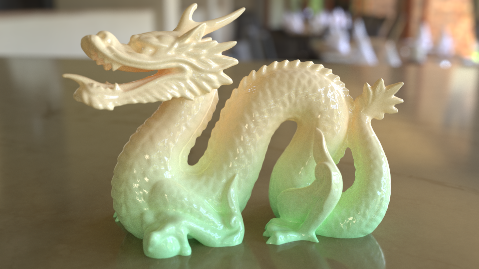
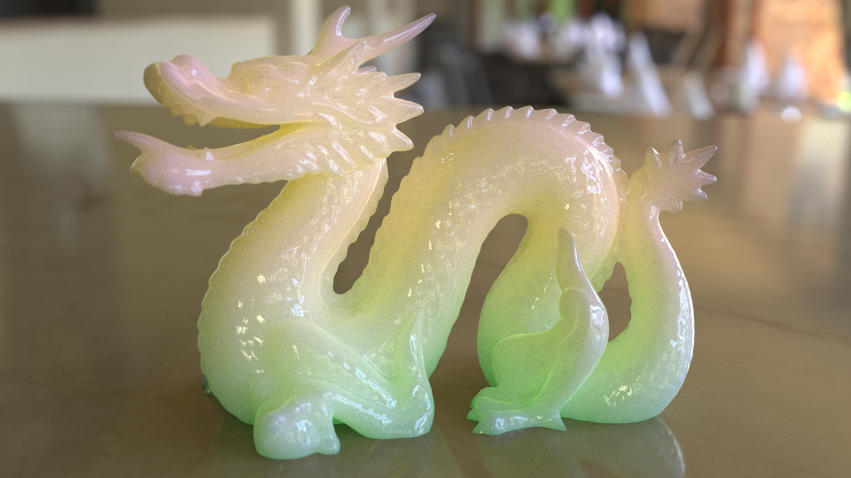
As we can easily see from the comparison, subsurface scattering shows a more waxy feeling, it feels more transparent than the Lambert BRDF. In a nutshell, subsurface scattering means the incoming light penetrates through the surface of an object and leaves from another position that may not be the same as the position where it enters the surface. The most common example in our everyday life is human skin. So the question is, what makes it a difficult challenge in computer graphics? If we get back to the rendering equation,

It is not hard to notice that there is no support for subsurface scattering in this equation at all since the whole integral is just about one single position. When we talk about BRDF, it is a simplified version of BSSRDF. We can treat BRDF as a delta function version of BSSRDF. If we look at the rendering equation in a more generalized way, it can be written like this,

As we can see, we gained two more dimensions by considering subsurface scattering. In other words, instead of just considering light coming from all directions at a single point on the surface, we also need to evaluate the contribution of light coming from all other positions. The direction domain is an isolated domain that is generally not affected by other factors. However, the same thing doesn’t go true for positions, which highly depends on the shape of the geometry, meaning accurate importance sampling position is a lot harder than sampling directions like what we used to do in BRDF evaluation.

And even if we have a good importance sampling algorithm, integrating the implementation with the existed path tracing algorithm that used to only consider BRDF also requires close attention to avoid mistakes that could accidentally introduce bias. A practical render engine also supports multiple layers of BSSRDFs, like Cycles. I also implemented the algorithm to support multiple layers of BSSRDF so that there is more flexibility of asset authoring.

Basic Idea of SSS

It makes very little sense to put down all of the math details of subsurface scattering here since there are already lots of resources available online. However, to avoid confusing readers, it is still worthwhile to introduce the basic concept briefly. Since I started by integrating PBRT’s implementation, the basic theory mentioned below is just a brief introduction to the implementation of SSS in PBRT 3rd edition. For a deeper understanding of the way it works, PBRT has a few chapters that have a pretty solid explanation of every single detail in it.

Whenever we have a new BRDF model, the two most important things we need to do are always to figure out a proper way to evaluate the BRDF and a solid importance sampling algorithm so that the implementation could converge efficiently. BSSRDF implementation sounded a bit intimidated to me at the beginning when I literally knew nothing about it. But the reality is that this is not that different from adding a new BRDF model, we still need to figure out a proper way to evaluate the function and an efficient importance sampling algorithm, for both direction and position. The only extra thing that is needed is to adjust the path tracing algorithm to make it aware of SSS and evaluate it when necessary.

Evaluating BSSRDF

This paper first introduced the model of separable BSSRDF to make things manageable. It achieved so by decoupling factors from each other. PBRT’s work is based on top of it.

With three parts in this model, the first part is responsible for accounting for the energy loss during light leaving the surface from inside. $ S_p(p_o, p_i) $ is mainly responsible for approximating the falloff factor due to the distance between $ p_o $ and $ p_i $ . Like the first part, the last one is for evaluating light energy loss due to light coming in through the surface.

The complexity of the simplified function is already a lot simpler with the approximation. To simplify things even more, $ S_p(p_o, p_i) $ will only consider the distance of the two input points instead of the relative positions with each other on the surface of the object. This greatly reduces the complexity of the problem again since BSSRDF will need no knowledge of the specific shape of the object, where the two points are lying on, to be evaluated. And this is what we usually call ‘diffusion profile’. A way to visualize it is to shoot a lazer thin ray on a totally flat surface with subsurface scattering. One nice thing about this simplification is that the model is independent of the specific model of diffusion profile, which means that we can choose whatever we want as long as it is normalized. Mathematically, the equation below needs to hold true,

Importance Sampling

Importance sampling of BSSRDF involves two things, sampling an incoming direction and sampling a position where the incoming light enters the volume of the SSS object from the surface. Sampling a direction is no different from sampling a direction using BRDF. As a matter of fact, PBRT uses a wrapper BXDF to hide the $ S_w $ part. And with the BRDF setup, it easily reuses existed code infrastructure to sample it.

Taking a sample around the point to be shaded is a bit more complex than taking a random direction around the same point since it depends on the shape of the geometry. There are numerous methods that can help to take samples. For example, in PBRT 2nd edition, they construct a KD-Tree for saving randomly generated points on the surface of the geometry. When taking samples, the algorithm can take advantage of the KD-Tree to ‘randomly’ pick nearby samples. The method that I choose to implement in my renderer is from this paper, which is also implemented in PBRT 3rd edition. The basic idea is to assume the geometry is totally flat and randomly pick a sample on the disk that floats right above the shading point. With the point picked on the disk, it then projects a ray (the green one) in the opposite direction of the surface normal at the shading point. The intersection of the short ray with the original geometry will be the sampled point.

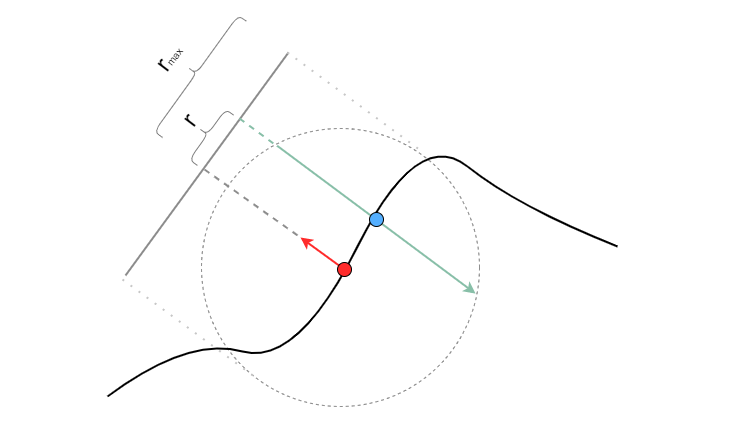
In the above image, $r_{max}$ is decided by the diffusion profile. And r is a random sample based on the chosen pdf. Luckily enough, the diffusion profile Disney offers in their paper already has a perfect pdf. One detail to be noted here is that we should have three $r_{max}$ because the diffusion profile has three channels. Here I assume we are not doing the real spectrum rendering. It is needed to pick one channel randomly first and having it taken into account eventually when evaluating its pdf.

The problem is more than what it appears to be in the above image. Whenever there is an assumption that breaks, problems arise. Of course, the geometries won’t be flat most of the time. Depending on the geometry and diffusion profile, there could be multiple intersections instead of just one. And also sometimes, when the projection ray is almost perpendicular to the geometry surface it intersects, it can result in fireflies. Those problems are addressed in PBRT 3rd edition. Please check here for further detail.

How Does It Fit in a Path Tracing Algorithm

In order to figure out how to integrate SSS implementation in a path tracer, it is necessary to know how a barebone path tracer works in general. My previous blog post mentioned some basics about it. Below is the pseudo-code of a minimal path tracer algorithm with BSSRDF in it.

color li(scene, ray, max_bounce_cnt){
    color ret(0.0f);
    int bounces = 0;
    auto r = ray;
    color throughput(1.0f);
    while( bounces < max_bounce_cnt ){
        // 1 - Get the intersection between the ray and the scene.
        //     Bail if it hits nothing. This is commonly the place to return sky color,
        //     while it is skipped for simplicity since it is not relevant.
        Intersection intersection;
        if( (intersection = get_intersect(scene, r)).IsInvalid() )
            break;

        // 2 - Construct BSDF
        intersection.bsdf = construct_bsdf(intersection);

        // 3 - Evaluate the contribution from light source
        ret += evaluate_light(intersection) * throughput;

        // 4 - Importance sample for the bounced ray
        float bsdf_pdf;
        vector dir;
        auto bsdf_evaluation = intersection.bsdf->sample_f(&dir, &bsdf_pdf);

        // 5 - Update throughput
        throughput *= bsdf_evaluation * dot(intersection.n, dir) / bsdf_pdf;

        // 6 - Update the bounce ray
        r = Ray(intersection.position , dir);

        // This is where we handle BSSRDF
        if(intersection.bssrdf){
            <<< Handle BSSRDF >>>
        }

        // 7 - Russian roulette. rand() returns value from 0 to 1 randomly and 
        //     the random samples are uniformly distributed.
        if(rand() < 0.3f && bounces > 3 )
            throughput /= 0.3f;
        else
            break;

        ++bounces;
    }
    return ret;
}

PBRT’s path tracing implementation is a lot more complex than the above code. But in order to keep things in control, I stripped the irrelevant parts with only the core left. To make it clear, basically, it does the following things inside the loop (pretending that there is no bssrdf)

1. For each ray, try getting the nearest intersection with the scene first. If the ray hits nothing, it will simply break out of the loop.
2. If there is an intersection found, it will construct bsdf, which commonly represents the material.
3. For a valid material, it will evaluate light contribution through the bsdf.
4. Importance sampling for the next ray based on the bsdf, this is essentially a greedy method.
5. Update the throughput value so that the contribution of the next light bounce will take this one into account.
6. Update the bounce ray.
7. Russian roulette to make things under control and unbiased.

This above logic is the very essential core of a path tracing algorithm with lots of detailed implementation skipped, for example like multiple importance sampling, sky rendering, volumetric rendering, efficient Russian roulette, etc. But this is more than enough as a playground for us to introduce how a BSSRDF can fit in it. In the case there is bssrdf available, we only need to implement the branch of the condition. Following is the code snippet of <<< Handle BSSRDF >>>.

// Take a random sample by projecting a ray.
Intersection bssrdf_intersection;
float bssrdf_pdf;
const auto bssrdf_evaluation = intersection.bssrdf->sample_s(scene, 
                               &bssrdf_pdf, &bssrdf_intersection);

// Bail if there is no intersection.
if(bssrdf_intersection.IsInvalid())
    break;

// Update the throughput
throughput *= bssrdf_evaluation / bssrdf_pdf;

// Evaluate direct illumination
ret += evaluate_light(intersection) * throughput;

// Take another sample of direction for the bounce ray.
float bsdf_pdf;
vector dir;
auto bsdf_evaluation = bssrdf_intersection.bsdf->sample_f(&dir, &bsdf_pdf);

// Update throughput
throughput *= bsdf_evaluation * dot(intersection.n, dir) / bsdf_pdf;

// Update the bounce ray
r = Ray(intersection.position , dir);

What it does is pretty self-explanatory. Below is a breakdown of computation it does in order to evaluate BSSRDF.

• It first takes a sampled position near the shading point. The importance sampling of the diffusion profile happens under the hood. One important detail to be noted here is that the interface sample_s will silently add a fake brdf in the bsdf of the intersection for importance sampling the ray direction of the next iteration in the loop.
• If nothing is found, it will simply bail. This will be a source of bias and it is why SSS evaluation tends to tint with a different color at the thin parts of the object.
• Update the throughput, this line will count the attenuation caused by the distance between the shading point and sampled point. It is essentially $ S_p(\omega_i, \omega_o) $ mentioned previously. Please note that the first Fresnel part is already handled in the BXDF right before the condition.
• Starting from here, we need to evaluate both direct illumination and indirect illumination to take both into account.
  • Direct illumination evaluation is fairly simple in the way that we can take advantage of the existed code infrastructure.
  • With the fake BRDF added previously, we can take a sample direction based on it. This direction will be used as the bounce ray for the next iteration in the loop.

There is a lot of mathematics to derive to further prove what the above code does makes sense. However, this is not the purpose of this blog. Instead of focusing on the mathematical theory, I would prefer to talk more about the real engineering problems that I encountered during my implementation. So I will stop introducing the basics here and move forward with talking about my iterations.

Enhancements

After my functional integration of PBRT’s subsurface scattering algorithm, I found that there are still more problems to solve.

• Sometimes there are too many fireflies.
• One SSS material can’t blend with other SSS materials.
• Subsurface scattering implementation is not flexible enough to be blended with other BRDFs.
• There is some space for better performance.

It appears that Cycles, the internal offline renderer in Blender, has a more robust implementation. Luckily, Cycles is also an open-source project. So I spend quite some time digging into what they improved over my integration from PBRT. With lots of iterations, my SSS implementation is a lot more robust than it was at the beginning.

Reduce Fireflies

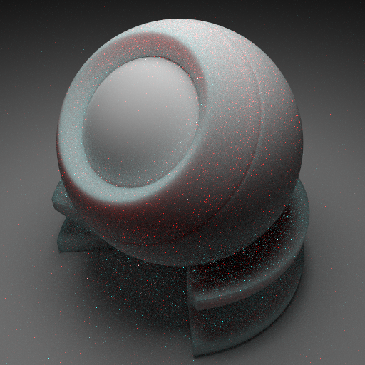
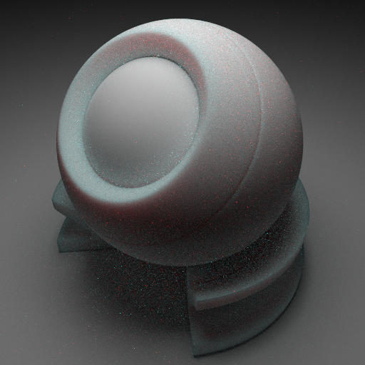
The first and most annoying issue that I would like to solve was the fireflies. These fireflies won’t simply go away as we bump up the number of samples per pixel. With the SSS integration in my renderer, this was what I got at the beginning. Please be noted that there is no coating layer and it is on purpose because I would like to avoid any other potential sources of fireflies. This is already 1k samples and even by bumping the spp up to 8k, fireflies won’t be totally gone, if not getting worse. The firefly problem renders the algorithm impractical in my renderer since it is so obvious. Of course, we can also rely on some post-processing, like a denoiser, to mitigate the problem. But it would be nice to know what the sources of the problems are and fix them for real.

Don’t Evaluate SSS Unnecessarily

One observation that I made during my iteration was that the impact of SSS objects on its neighbors with SSS materials is very close to what a Lambert model has. Taking the advantage of the assumption, I chose to silently replace SSS objects with lambert if the previous reflection model has SSS. Below is a comparison of the same shot with and without the trick, the difference is barely noticeable to me. It is worth mentioning that I clamped pixels with high radiance value to avoid fireflies in both shots.

Allow SSS to SSS bounces

Disallow SSS to SSS bounces

Clearly, this will avoid some importance sampling of BSSRDF and converts a BSSRDF to a simple lambert model. Most BXDF importance sampling algorithms are commonly done locally without the knowledge of the surroundings. Importance sampling algorithm used to randomly sample points on its nearby surfaces in this SSS implementation involves shooting short rays. This is easily an order of magnitude more expensive than BXDF’s importance sampling algorithm. However, given the rare cases where there are two consecutive SSS bounces in the same path, the differences in terms of computation in a practical scene like the above are close to minimal. In some cases where SSS surfaces face each other, there is a greater chance for a path to have multiple consecutive samples on the same mesh with SSS. For example, like the one shown below. Even in these cases, the performance gain is not too much, roughly 10% reduction in rendering speed. However, the biggest gain in terms of performance is that it opens a door for our next iteration by making it possible, which we will cover later.

After

Before

The above two shots are rendered both with 1024 samples per pixel. We can easily notice that the optimization turns out to be very effective in terms of reducing fireflies, which was my primary reason for considering implementing it at the cost of slightly extra biased results. Even with the SPPs bumped to 8k, the fireflies still doesn’t go away in the original implementation. With the optimization, it almost gets rid of more than 90% of the total fireflies at no performance cost. And we saw from the bunny example, it doesn’t have a big impact on the final result. Of course, we can argue that the SSS to SSS bounces is not as many as it is in this example, the visual comparison of those shots may not represent the biggest potential bias we could eventually get. But since the SSS algorithm has some pretty aggressive assumptions made at the very beginning, I would be willing to sacrifice a bit of accuracy to implement a reasonable SSS algorithm with limited fireflies.

What Happens Under the Hood

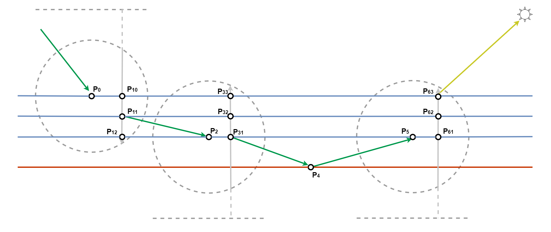
I think it is worth a little bit of explanation here to make it clear why such a trick can get rid of the majority of the fireflies. To answer the question, it is necessary to figure out where do these fireflies come from? By taking a deeper look into what happens here, I noticed that the volume inside the outer ball is not empty at all. It has multiple layers of geometries. Following is a demonstration of what could happen inside the volume of the outer ball. Of course, there are no three parallel surfaces in the outer ball mesh, but it does lead to rays bouncing between its surfaces, so this representation doesn’t lose its generality. Upon the first intersection of the primary ray, it will pick three samples on the surface of the objects, some of which happen to be inside the volume and is kind of unfortunate. It is unfortunate because the next sample it picks will also be from the exact same material with SSS. As we can see from the path $ P_0 \rightarrow P_{11} \rightarrow P_{2} \rightarrow P_{31} \rightarrow P_{4} \rightarrow P_{5} \rightarrow P_{63}$ , which is essentially three bounces. Please be noted that the transition from $ P_0 $ to $ P_{11} $ is not considered a bounce, it is just taking a sample of BSSRDF. Same goes true about the transition from $ P_5 $ to $ P_{63} $ . The real problem behind this is that every single path is trying to make its way out, while only a very minority group of lucky paths will make it. However, the ones made out will make an excessive amount of contribution to the evaluation since their PDF is extremely low. In practice, the situation is way worse than just a few bounces. I think there are a few reasons for this problem,

• Unnecessary complex internal structure of the outer ball. There is no real solution for this unless we ask data authors to change the way they do things, which could be a big limitation to artists.
• The distance profile is nowhere near being physically accurate. There is also no easy solution for this one. It because is those bold assumptions that make this algorithm feasible.
• Importance sampling does not always stick to the target function, which is the distance profile. Although the Disney distance profile can be analytically sampled with a perfect PDF, the unknown shape of geometry easily makes the sampling algorithm less efficient. We will cover it later.

Replacing SSS with lambert if the previous material has SSS will almost prevent this from happening. Because the path will be blocked when going from $ P_{11} $ to $ P_2 $ . Rays won’t bounce between complex meshes with SSS materials. Of course, light does bounce between complex shapes with SSS materials in reality, but without a good importance sampling algorithm and distance profile, this will easily lead to fireflies. And considering the multi-bounces inside SSS materials don’t have the biggest impact on the final visual, I chose to ignore it by replacing SSS with lambert if necessary.

The Catch of Replacing SSS with Lambert

Given a specific path, depending on the direction of evaluation, the end result of rendering equation evaluation could be different. Imagine there is a path like this $ E \rightarrow A \rightarrow B \rightarrow L $ , where E stands for eye, A and B stand for two points on surfaces with SSS, L represents light. If the direction of evaluation is from the eye to the light, A will be evaluated with SSS model, but B will be a lambert model. While if the direction of the evaluation goes the other way, B will be evaluated with SSS, and A will be simplified with lambert model. This clearly introduces some bias between path evaluation from different directions. This might not be a problem at all for unidirectional path tracing or light tracing, where evaluation is always one direction. For algorithms like bidirectional path tracing, this will introduce an extra layer of bias. Same reason here, considering the multiple sources of biases in the algorithm, I don’t mind having another one here.

Evaluate at all Intersections

The above-mentioned trick allows the algorithm renders with SSS in a way that converges a lot faster. Clearly, this is not a flawless solution since there are still quite some fireflies in the shot. These fireflies must come from other sources in the sampling process.

Fireflies commonly show up whenever the importance sampling algorithm is not very efficient. In the beginning, I didn’t choose to believe it since that diffusion profile from the Disney paper has a perfect pdf function. However, after taking a deeper look into the process, I found a problem that could cause it.

There are clearly some other factors that will affect the efficiency of the importance sampling, like the light source. It would be very hard, if not impossible, to take lights into account when taking samples with importance sampling algorithm. But the multi-intersection nature of the algorithm does lead to some problems. Like we mentioned before, there is a possibility that the projection ray will hit multiple surfaces with the same objects, instead of just one. In these cases, PBRT will choose to uniformly pick one random intersection and divide the diffusion profile PDF by the number of intersections that the short ray hits in total. This essentially adds a weighting factor for the original pdf. Mathematically, the final pdf should be as below,

R is the distance between the sampled point on the disk to the center of the disk. X is the index of the point it picks among all intersections. So we can clearly see from this equation, the Disney importance sampling pdf is just one part of the final pdf we have. The second pdf uniformly takes one intersection among all randomly, it is a conditional probability distribution. And it is the efficiency of the final pdf that matters. Even if the first pdf is a perfect match of the original diffusion profile, the second extra pdf does have a chance to make it way less efficient. Not to mention, the first pdf is only a perfect pdf considering flat surfaces.

To explain it in a more intuitive way, if we look at the image below. The chances of sampling both red and green short rays are exactly the same since their distance to the center of the disk is the same. However, we have five times more chances of picking the red point than any of the green ones even if the red point has more distance compared with any of the green ones. To manually make things worse, if we place a light source near one of the green dots. We will have a much bigger contribution by picking the green dot that is near to the light source with a five times lower chance of picking it. This is a very typical example of why this importance sampling algorithm is not efficient in some cases. It can even get worse in practical situations.

It would be very hard to uniformly sample all intersections in this algorithm globally since we don’t know how many intersections there will be in total. The truth is there is not even a number, it is a continuous domain. But one thing that we can do to mitigate the problem is to avoid randomly picking one intersection among all but to evaluate all of them. This was not possible before the first iteration since rays will grow exponentially without the above trick. But since I have it implemented, I can totally consider evaluating all intersections instead of just randomly picking one of them. Following is a comparison of the shots with and without this method, it is obvious how efficient it is after this iteration. It is worth noting that instead of having the same spp this time, I choose to configure the settings differently so that the rendering time is roughly the same, which makes the comparison fairer.

After

Before

Given the result of the shot, I can hardly tell any firefly in it. This is already a firefly free solution to me.

No Fresnel above SSS material

It is common that renderers will introduce a coating layer to simulate a glossy surface with SSS under it to deliver a wax-like feeling. PBRT uses fresnel to pursue better physically-based accuracy. But it is also not uncommon to see articles mentioning SSS without the fresnel part. Strictly speaking, subsurface scattering should have no connection with the coating layer since they are not tightly couple all the time. Also, because I have my plan to support flexible blending between bssrdf and bxdf in my material system, which will be covered later in this blog, I can totally approximate the fresnel part in my shader, instead of hardcode it in the bssrdf.

Ideally, my goal here is to make sure I can guarantee this equation,

The benefit of securing such an equation is that it allows me to have a proper transition between sss and lambert model without introducing a noticeable boundary in between. This doesn’t sound like a big deal, but it does offer a bit more flexibility of data authoring. For example, the shots below clearly demonstrate the differences. The mean free path goes to zero gradually as the position goes lower, eventually reaching zero somewhere around the neck of the monkey head. It is not too obvious, but we can notice the line at the bottom of the monkey head by taking a closer look. This is because the above equation is not true for the original implementation.

Smooth Transition

No Smooth Transition

The way I achieve this smooth transition is by killing the two Fresnel parts and adding a denominator of $ \pi $. So the equation of my BSSRDF goes like this,

As the mean free path length approaches to zero, the $S_p(p_o, p_i)$ becomes linearly proportional to dirac-delta function. Also, as we know, a dirac-delta function will simplify integral in Monta Carlo estimation by dropping one dimension. The constant factor is what we need to figure out here. Since the pdf, which is proportional to this BSSRDF, the only difference between this BSSRDF and the pdf is the color tint part. Because when the mean free path approaches zero, it is very likely there is only one single intersection. This means that we don’t need to take the conditional probability density function into account. So the pdf and bssrdf have this connection

By taking a look at the Monte Carlo estimation, we got this

And dropping this equation back to the one we want to fulfill, it is obvious that this is a perfect match, which is also proved by the above shot.

Avoid Finding Intersection with other Meshes

One detail in SSS implementation is to tell whether an intersection is a valid one during importance sampling of nearby positions. PBRT considers it a valid intersection as long as the material is the same. In case there are two meshes with the same SSS material, they will find intersections on each other, which will result in incorrect approximation.

In my renderer, I chose to instance subsurface scattering materials so that each mesh object has its own material instance with a unique id. This will avoid the problem. A material instance is just a thin wrapper of the original material, the memory overhead is close to minimal in most cases.

Refactor Material System in my Renderer

Prior to implementing sss in my renderer, it used to only have a linear combination of BXDFs in a data structure called BSDF. Strictly speaking, it is not just linearly blended BXDFs, since some BRDF, like Coat, can take a BSDF as an input argument. This converts the data into a tree. But this is irrelevant to the topic in this blog, we can ignore it. To extend the system with sss features, I added a pointer for each material so that they can access more than BSDF data. This can be easily integrated in the above pseudo-code. However, there are some limitations with this implementation.

• If a material has BSSRDF, it won’t be allowed to have other BXDF that is not relevant. The algorithm won’t work very well. It will always pick BSSRDF if one existed. This limitation means that we can’t blend BSSRDF with other BXDF stored in the BSDF.
• The system can only have one single BSSRDF since there is only one single pointer holding it. But sometimes, we might want to have multiple diffusion profiles blended together to achieve better subsurface scattering results, like skin rendering. The current system clearly doesn’t offer this flexibility.

In order to support flexible blending between BXDF and BSSRDF, I chose to refactor my material system. As we know that BSSRDF is a generalized version of BXDF. One option would be to derive all BXDF implementations from BSSRDF. This does stick to the truth in reality, but it immediately raised some problems in terms of coding. I don’t particularly like the design of this idea for two reasons

• The interface will be fatter with more arguments since we have more dimensions in BSSRDF. It might lead to less performance due to more arguments in call stack and in most cases where there is no subsurface scattering, lots of the arguments are not even used at all.
• The path tracing, bidirectional path tracing algorithms will have to treat everything like a BSSRDF, which won’t be efficient in terms of performance.

Eventually, I ended up with the other solution, both BXDF and BSSRDF derive from what I call scattering unit. All scattering units are held in a structure named scattering event, which is what I used to replace BSDF in my old system. The biggest difference introduced here is that scattering event can also hold multiple BSSRDFs along with BXDFs. A subtle difference here is that instead of holding an array of scattering units, the scattering event data structure chooses to hold two separate arrays, with one for BXDFs and the other for BSSRDFs, since they behave very differently compared with each other. This way it allows me to put the interfaces of BXDF and BSSRDF one level lower than their base class.

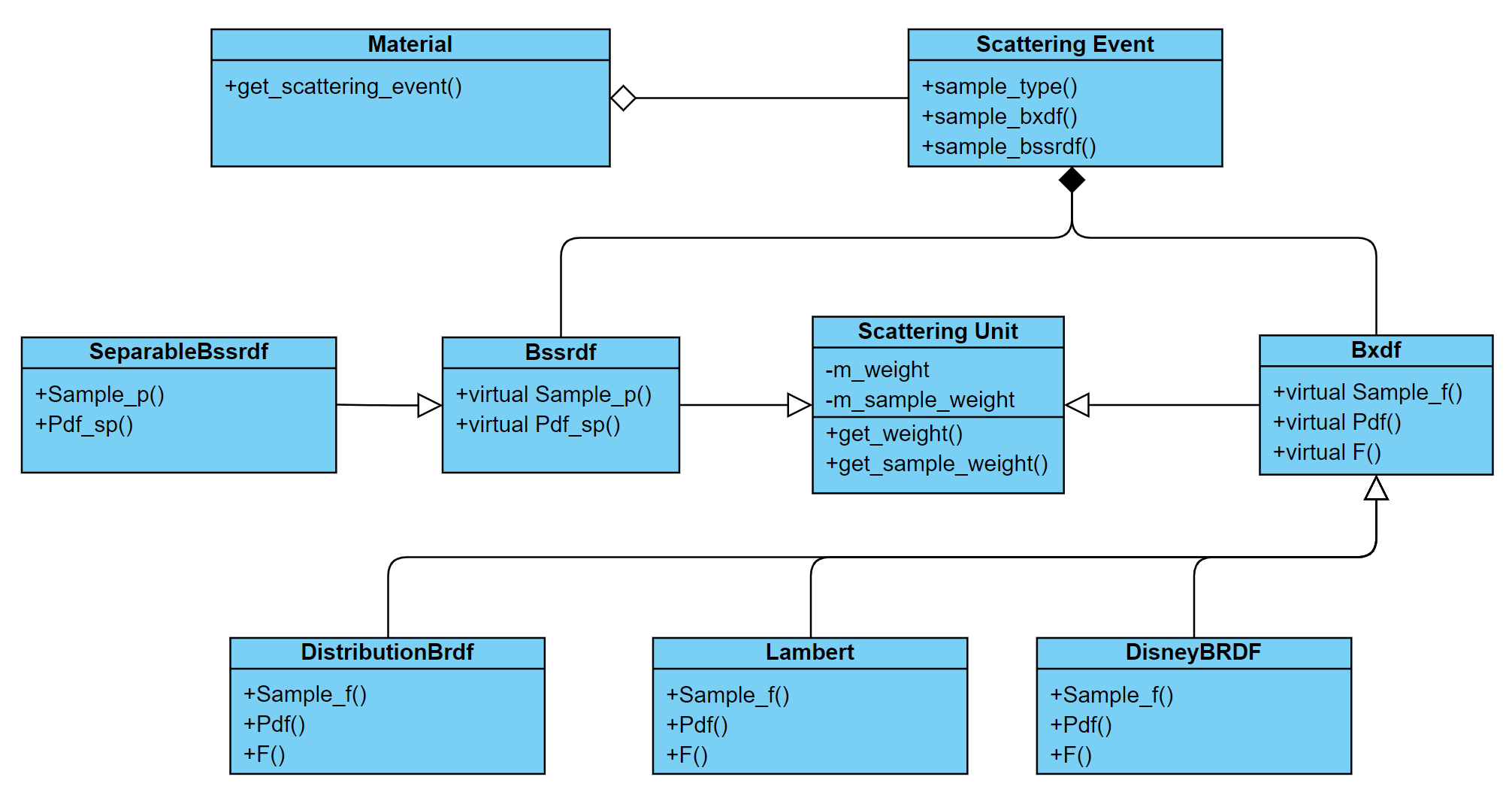
Above is a simplified class diagram that demonstrates what I implemented in my renderer. It doesn’t have everything I have done in it. For example, there are only three BRDFs shown in this diagram, while I have implemented a lot more than this. However, it gives a good explanation of what the big picture is.

Again, there are a few adjustments needed to be done in my path tracing algorithm

• In the third step shown in my pseudo-code, where we used to only evaluate BRDFs. We can choose to randomly pick one scattering unit from scattering event. The scattering unit can be either a BXDF or a BSSRDF. If a BXDF is chosen, we still stick to the old path. In the case of a BSSRDF chosen, the new algorithm will pick sampled positions and evaluate all of them to approximate the contribution from direct illumination.
• Just like what we did for step 3, we need to do similar things for step 4, where we used to only take direction samples from BXDF. Again, we randomly choose to have one scattering unit among all in the scattering event. If a BSSRDF is chosen, we first randomly pick a sampled position based on the BSSRDF model, and then we will recursively evaluate the indirect illumination for this part.

These two steps are what I eventually did in my renderer. But I guess it is also possible to merge the two steps in one by randomly picking between BXDF and BSSRDF once. Once one is picked, we use the type for both evaluation and importance sampling. I haven’t tried it in my renderer, it sounds to me it could work. There might be other problems though.

Ideally, I would like to put the pseudo-code here too. But in order to avoid a too much longer post, I chose to skip it since it is not that hard to implement. For anyone, who is interested, here is the implementation in my renderer.

Multiple SSS

Single SSS

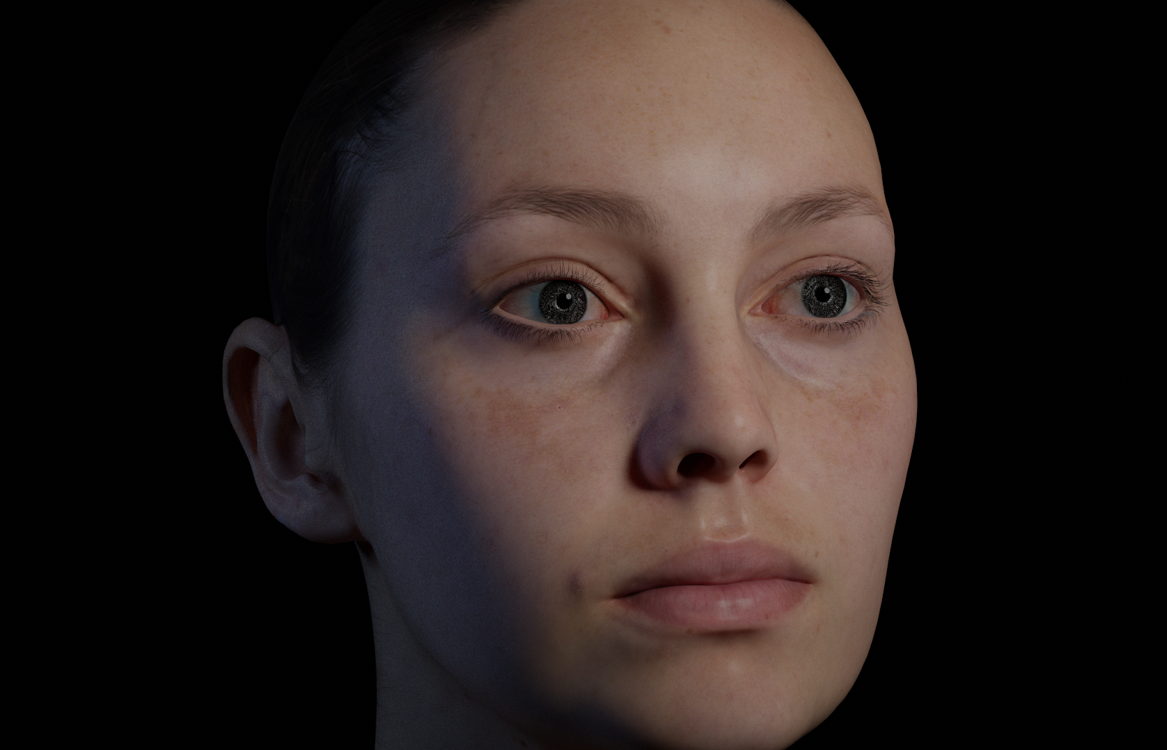
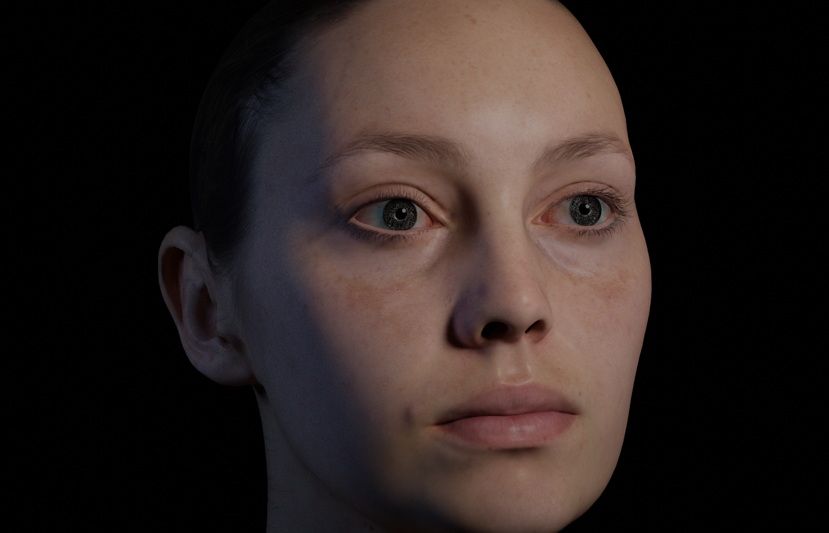
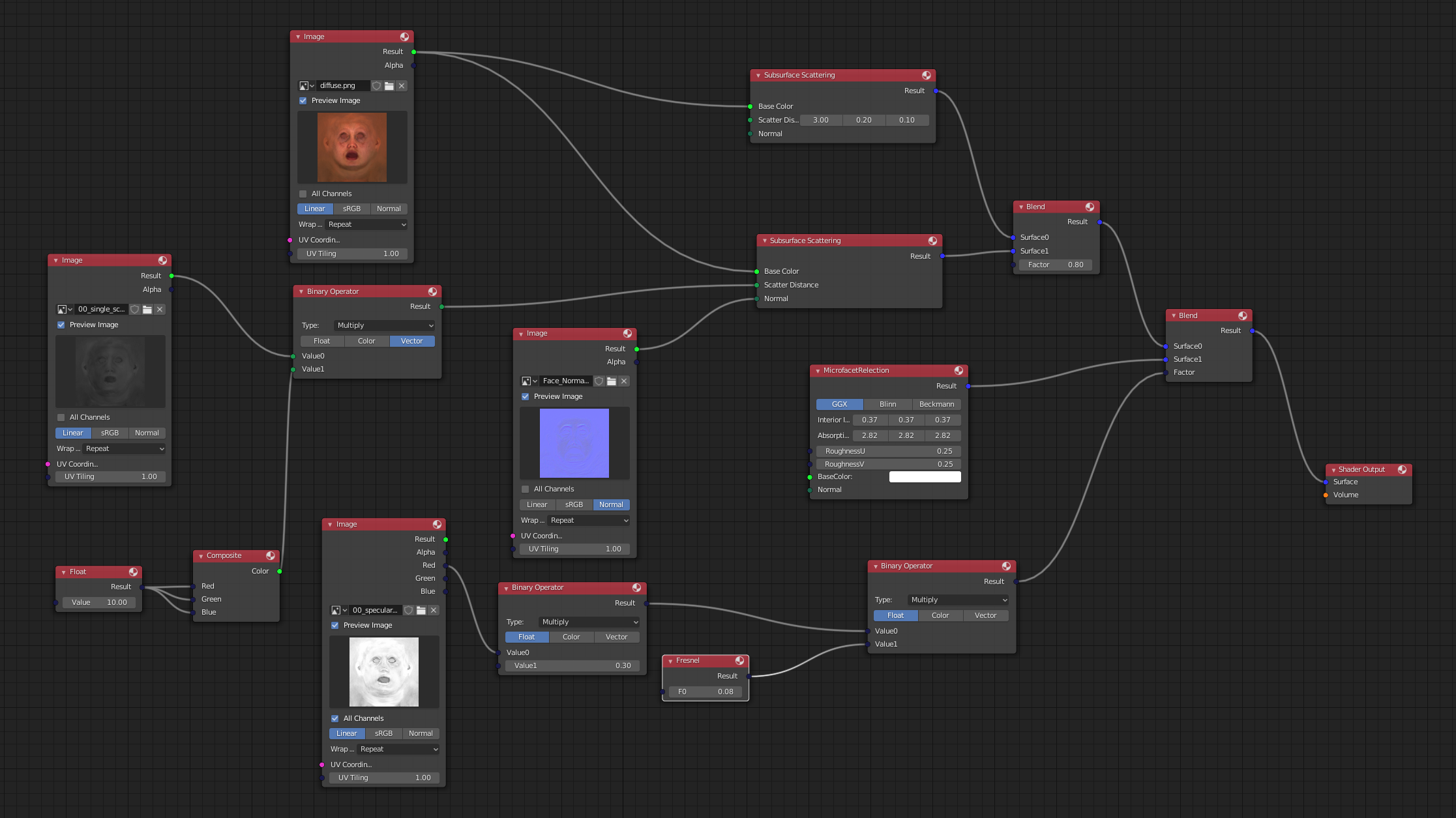
Above is an example that uses this feature to implement a skin shader. The comparison is single subsurface scattering versus multiple subsurface scattering. The difference is very subtle, but it is visible in the dark area on her face. Also, apart from blending subsurface scattering, this material also blends sss with regular brdf to simulate a bit of specular light on her face. Below is the shader graph of this material used to render the shot. Click it for an enlarged image if it is not clear enough.

Optimizations

Besides the enhancements that I did in my implementation, I also made a couple of optimizations that purely aim at improving performance. They don’t contribute to convergence rate or image quality that much, but making things faster is already a good reason to check them in.

Intersection tests

SSS implementation mentioned in this blog requires finding the intersections with K nearest primitives. A naive way to get it done without introducing more complexity is to find the nearest intersection first and then adjust the ray origin a little bit off the surface along the ray direction, get the next intersection. The process keeps going until either K nearest intersections are found or it exceeds the allowed range of our interest. This naive implementation is simple in the way that it doesn’t require any changes in the spatial acceleration structure. The algorithm to find the K nearest intersection is totally limited in SSS implementation itself. While it does comes at a cost of performing duplicated evaluation multiple times. Imagine in a case, where there are only five primitives in a leaf node, all of which intersect with the ray to be tested, and they are also the first five intersections. If our K is 4 in this case, we will have to perform the ray primitive intersection 20 times just to get the nearest 4 intersections in this leaf. This doesn’t even count the workload to iterate the traversal to the leaf node, which is also duplicated by 4 times.

A slightly advanced approach to solving this problem is to introduce a dedicated interface to return K nearest intersections along the ray. This does require keeping a list of intersection history, which takes a bit of extra memory during intersection evaluation. But it efficiently avoids all the above-mentioned duplicated computation during finding the K nearest intersections. In my renderer, I chose to implement the algorithm in all of my spatial data structures, including kd-tree, BVH, OBVH, QBVH, uniform grid, octree.

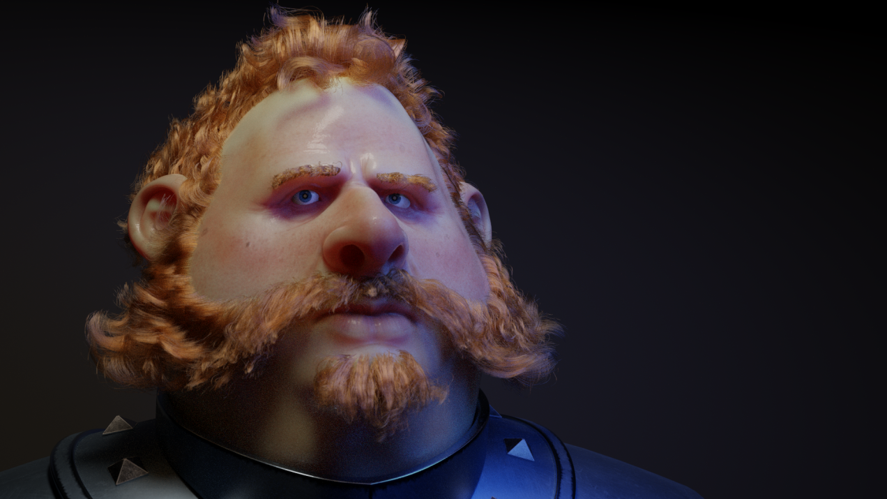
Above is another example generated in my renderer. A big proportion of the image is covered by skin, which is essentially this subsurface scattering model. But apart from these skin pixels, there are also other materials like metal, hair, and even a different primitive type. In such a scene, this optimization reduces the total intersection by 14%, eventually improves the final rendering performance by 11.5%. For a pure subsurface scattering scene like the monkey head shot, performance gain can be as high as 14%.

Avoid MIS

Whenever we find an intersection to keep iterating, we need to evaluate how much light coming in through that exit point. Normally, we will take multiple samples from both light sources and the BRDF to avoid bad sampling, which could be caused by either a spiky shape BRDF or a tiny light source. But we know for a fact that the BRDF here is lambert, there is no need to take samples from BRDF at all. The thesis that introduced multiple importance sampling already made it clear that MIS doesn’t necessarily improve quality all the time. We can simply take advantage of this to avoid taking unnecessary samples. Taking samples from light sources works simply well enough.

Ideally, this should get less shadow ray since MIS will require two separate shadow ray to be shot while sampling the light source only needs one. And this should mean that we have less computation to do. Also, in the case of very small area light sources, MIS may have a slightly worse result than sampling light direction only since sampling from lambert brdf will almost always miss the light source. However, my experimental data doesn’t indicate too much gain from this optimization. I still kept it in my renderer since I can’t justify any reason to take samples from brdf in this case and at least it doesn’t hurt anything.

Miscellaneous

Apart from the above few optimizations I made, there are also some minor optimizations I did in my renderer. They are not that important, but it is nice to have since they are fairly easy to implement.

• Ignore SSS after too many paths
  Just like we have the maximum bounces of the main path, we can totally have another sperate control purely over subsurface scattering materials. This is just another finer control over the system.
• Avoid generating SSS when mean free path is 0 in all channels
  Generally, subsurface scattering evaluation has a different branch in path tracing algorithm, which is more expensive in terms of performance. With the proper transition feature, I would prefer to silently replace them with lambert whenever mean free paths are zero. This is no catch of doing so.
  Another further optimization could be partially replacing subsurface scattering with lambert when the corresponding channel has mean free path that is zero. This idea takes advantage of the blending system that I did in my render so that it can blend a lambert with a subsurface scattering together.

A Failed Attempt

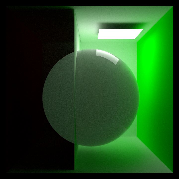
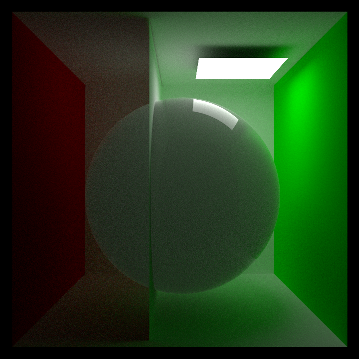
A more aggressive way is to ignore SSS from all BRDFs without spiky shapes, like lambert. This might sound like a reasonable optimization at the beginning. But it will destroy some nice things SSS delivers, like the color tint in the shadow of the second shots I showed in this blog. A more extreme case is like the two shots below. Though these are not the best demo cases for showing SSS features since both of the spheres look fairly flat. But it does clearly demonstrates the potential problem that could result from such aggressive optimization. With a concrete wall roughly in the middle of the Cornell box, the sphere with SSS material is pretty much the only way that light can path through from the right side of the Cornell box to the left side. If we ignore SSS from all non-spiky shape BRDF, we will lose all light contribution on the left side of the Cornell Box. Another slight subtle difference is the top right corner gets a bit stronger bounced light contribution. This is probably because SSS will lose some energy when it fails to find samples on the surface of the same mesh object. I can’t say I care too much about the brighter bounce, but I definitely don’t like losing the nice feature of allowing light penetrating through SSS objects. Eventually, I didn’t choose to implement this in my renderer.

No SSS after Lambert

Regular

Even if I would like to implement it, there is another problem. It is not entirely straightforward to categorize materials based on how rough they are. PBRT has a hardcoded category for each of its BRDF. However, the ones like measured BRDF, will be very difficult to be hardcoded. Not to mention there are things like Disney BRDF, which offers lots of flexibility with a gradual transition from being rough to smooth. An even more extreme case is a rough material with a smooth coating layer on top. There is just not a clear boundary between rough materials and smooth ones.

Summary

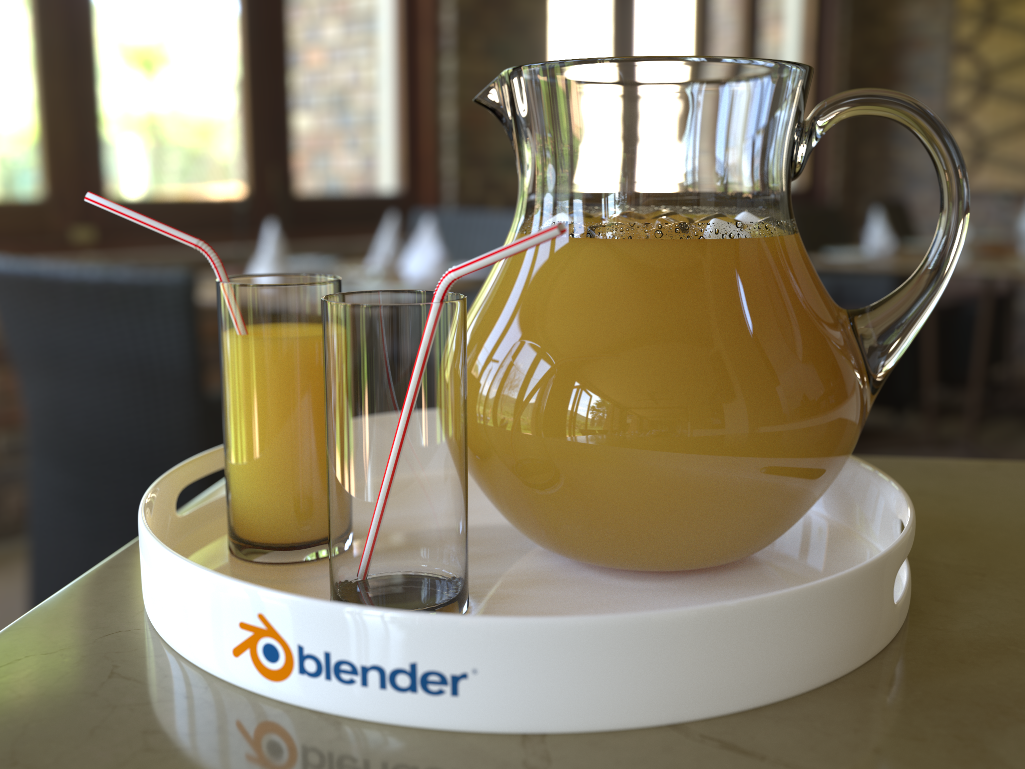
In this blog, I mentioned my iterations during implementing subsurface scattering. These iterations allow me to render subsurface scattering in a more efficient way. Apart from the common subsurface scattering materials, like skin, wax, this algorithm can also be used to approximate juice sometimes, like in the image below. I believe there could be a better way to render this, but it is always good to know more applications of the algorithm.

However, there are still some unsolved problems remained and potential improvements to be done in the future,

• A separate spatial structure for each object with subsurface scattering will skip all of the traversal steps from the root all the way to the interior node that holds the object.
• It is not hard to notice that this algorithm will fail to converge to the correct result when the geometry is thin. For example, the head of the dragon shot is a bit dark because most short rays end up finding nothing, while they still have valid pdf. Somehow, Cycles solved the problem, it would be worth investigating.
• Subsurface scattering is not supported in my bidirectional path tracing algorithm. Adding support to it does sound challenging since bdpt is not an easy algorithm to start with. Making sure all MIS weights are correct while adding sss would be difficult.
• There are also numerous other methods for rendering subsurface scattering, like random walk sss. It would be fun to dive into the other algorithms and know the trade-off of these algorithms too.

References

[1] Approximate Reflectance Profiles for Efficient Subsurface Scattering
[2] BSSRDF Importance Sampling
[3] Physically based rendering
[4] A Practical Model for Subsurface Light Transport
[5] Separable Subsurface Scattering
[6] Advanced Techniques for Realistic Real-Time Skin Rendering
[7] Cycles Renderer
[8] A Practical Model for Subsurface Light Transport
[9] An Introduction To Real-Time Subsurface Scattering
[10] Efficient Screen-Space Subsurface Scattering Using Burley’s Normalization Diffusion in Real-Time
[11] Basics about path tracing
[12] Robust Monte Carlo Methods For Light Transport Simulation