Procedural UV Derivatives Evaluation in SORT Renderer
In this post, I want to talk about a topic I have been meaning to write about for quite a few years: texture UV derivatives evaluation in my offline renderer, SORT (Simple Open Source Ray Tracer), which I’ll use throughout this post. It normally is not a major challenge. However, my own custom shading language[1] specifically designed for my renderer adds quite a lot of complexity in it. It was previously named as Tiny Shading Language and renamed as SORT Shading Language (SSL for short) as I fused it into my rendererer project. This article may not be useful to everyone, but it should be relevant if you are interested in implementing an offline renderer and shading language yourself. If that describes you, I hope this post is useful, because this particular combination of topics is rarely discussed in one place.
Why Do We Care?
Derivatives are a powerful mathematical tool used widely across many scientific fields, such as deep learning, physics, biology, and many others. At first glance, they do not seem like a must-have for computer graphics. In practice, you can build a toy offline renderer that produces great images without them. SORT renderer used to lack derivative support entirely, yet it could still render respectable results.
As a matter of fact, derivatives do show up throughout computer graphics in many places. Signed distance fields (SDFs) use them to approximate surface normals. Geometry processing often relies on them for operations like smoothing and deformation. Smoothed particle hydrodynamics (SPH) methods simulate fluids with them[2]. Gradient-domain rendering is another interesting area built on the same foundation[3]. The Jacobians in ReSTIR’s shift mapping are essentially derivatives as well[4]. The list goes on. Still, the application every graphics programmer knows best is mipmapping and that is the main reason I spent so much effort figuring out how to evaluate derivatives in my offline renderer.
Coming from a real time rendering background, I want to start with mipmapping in that context. Mipmapping is essential in real time rendering because it helps avoid texture aliasing. To hit real time frame rates, renderers can usually afford only a very limited number of samples per pixel, often just one. In fact, most modern game engines also use some form of upscaling[5, 6], which further lowers the effective sampling rate per pixel. With such a low sampling rate, any frequency above the Nyquist limit must be prefiltered to avoid artifacts. That is what mipmaps provide. They also help performance. Lower mip levels use less texture memory, are more likely to stay in the GPU cache, and can speed up texture sampling.
As useful as mipmaps are in real time rendering, their benefits are less decisive for offline renderers. Most Monte Carlo path tracers fight noise by increasing sample count, so with a much higher effective texture sampling rate, prefiltered textures matter less. Lower mip levels can still improve cache behavior, but that alone is not why production offline renderers invest in mipmapping.
There is another wrinkle. Mipmapping is not strictly unbiased. Even when the correct mip level is chosen from texture coordinate derivatives, filtering still introduces a small amount of error in theory. One source of bias is geometric, the sampling footprint induced by a path is rarely an axis aligned square in texture space, so approximating that footprint with filtering on a mipmap pyramid is not exact in general. Even when the footprint is axis aligned, if its boundary does not align exactly with a mip level’s texel grid, we usually blend the two nearest mip levels. That interpolation approximates detail between mip resolutions with a linear blend, which is typically biased. Setting that aside, consider an idealized setup, an orthographic camera, a viewport that matches a single quad (two triangles), and a texture with twice as many texels as screen pixels along each dimension. In that simple case, we should select the second most detailed mip level. To make the remaining bias concrete, suppose albedo is the product of two same-resolution textures, $T_A$ and $T_B$, with UVs $(u(x,y), v(x,y))$ at image location $(x,y)$. In theory, the integrated shading result is:
Note that $f$ could simply be a function of $(x,y)$ in the equation above. I write it with explicit texture lookups because that form makes the comparison to the mipmapped case clearer.
With prefiltered mipmapped lookups at the second most detailed mip level, each texture is averaged over the pixel footprint $\mathcal{P}(x,y)$ in texture space before they are multiplied, giving
It is apparent that $F_{\mathrm{mip}}$, the value obtained with mipmap filtering, is biased relative to $F$. Mipmapping is not unbiased, and unbiased estimation is critical in offline rendering, so production renderers need a compelling reason to use it anyway.
The main reason most commercial offline renderers adopt texture mipmaps is memory consumption. Instead of loading every texture at the start of a render, which is what most toy offline renderers do, a production renderer often touches only a tiny fraction of the data needed for the full image. During path tracing, when a mip level is requested, the renderer first checks whether it is already in the texture cache. If it is, it fetches the data and continues, much like a simple ray tracer. If not, the requesting thread is paused while an I/O thread loads the data from disk, and another worker can use the core in the meantime. When the load finishes, the original thread resumes. That may sound like overhead, but if physical cores stay busy and thread switching is cheap, which can be achieved through fibers[7], this cache can greatly reduce the texture memory needed to render a frame. In effect, the theoretical upper bound on memory usage for a shot is not only determined by asset size, but also output resolution[8, 9].
A texture cache in an offline renderer frees artists from being constrained by physical memory, it is possible only a fraction of the textures on disk is actually needed for a given shot. When the cache budget is exhausted, older data is evicted to make room for new requests. Mip levels that are never sampled are never loaded at all, which sharply cuts the renderer’s memory footprint. The cache budget still matters, you want enough headroom to avoid thrashing, but the system makes it practical to render scenes whose total texture data far exceeds the physical memory of the machine doing the work.
Texture coordinate derivatives determine which mip level to use for a given sample and therefore govern filtering quality. Because a texture cache loads mip levels on demand, the cache relies on accurate derivative estimates, incorrect derivatives cause over-filtering or under-filtering and can force unnecessary loads or evictions. Reliable derivative evaluation is thus a prerequisite for combining mipmapped textures with a paging cache, a requirement that motivates the work described in the remainder of this post.
Challenges in SORT Renderer
UV coordinate derivative evaluation is not rocket science, but it does require some calculus. There were several articles on evaluating UV derivatives in Ray Tracing Gems II[10, 11, 12]. Many open source renderers, including PBRT[13], also use partial derivatives for mip selection. On the surface, the problem does not look complicated.
To fully understand why this becomes a major challenge in SORT, it is important to understand the rationale behind how SORT processes materials in the first place.
Material System in SORT Renderer
Ever since I built a Blender plugin for SORT, I realized the renderer needed a shader graph based material system. It was an interesting challenge at the time, and such workflows are common in both film and games.
In game industry, engines typically gather all nodes and emit a single shader kernel (possibly split across several files) for the shader compiler. From the compiler’s perspective, there is no shader graph, only shaders. Though not every game engine uses shader graphs. For example, Naughty Dog’s in-house engine uses shader packages[14]. Offline renderers often take a different path. Open Shading Language accepts shader segments, and the compiler wires them together according to the host program. In effect, the compiler does the gathering, not the rendering engine. Other compilers may work differently. I do not have full visibility into all of them.
Initially, I used OSL in my renderer, then introduced my own shading language. A primary motivation was Apple Silicon support. At the time, OSL had no official Apple Silicon build, and it was unclear when that would arrive. By piggybacking on LLVM, I implemented a compiler that targets multiple CPU architectures (x64 and Arm64) and operating systems (Windows, Ubuntu, and macOS). Below is a brief overview of how SSL fits into SORT.
- The Blender plugin exports shader segments as source code into a binary asset file based on material shader graph information.
- It then spawns the renderer with an argument pointing to that asset. This step can run asynchronously.
- During startup, SORT walks materials like other renderers, but instead of loading baked parameters from the asset, it loads shader code, similar to how real time engines compile HLSL. SSL compilation runs in a multithreaded environment. Each material stores the resulting JIT compiled function pointer.
- During path tracing, whenever a material is needed, the renderer invokes that JIT compiled function, transferring control from C++ to compiled SSL code.
- For texture sampling, SSL calls a C++ interface defined by SORT so the renderer handles sampling details.
- This is intentional. Decoupling texture sampling from SSL leaves room for a texture cache system later, which would require pausing threads, outside SSL’s scope.
- After any texture sampling, SSL resumes, completes its instructions, and returns a closure tree to the renderer. That tree becomes a BSDF, a stack of blended BxDF layers. Parameters such as albedo and roughness are evaluated entirely in SSL, which is its main purpose. The renderer then continues like any other path tracer.
As this workflow shows, SSL works in a similar fashion to OSL. It takes shader segments and wires them together. Its role is to move BxDF parameter evaluation from a hard coded fixed pipeline into artist programmable logic, not to own lighting or shading, despite the name “shading language”. Those parameters can depend on texture lookups, which in turn depend on UV coordinates, which ultimately depend on SSL’s global inputs. SSL global structure is an analogue to root signature concept in D3D12, it is a structure that passes data from the renderer (C++) into the shader (SSL). The exact formulas for texture coordinates are authored during content creation, not fixed at renderer compile time. That separation is the root cause of the UV derivative challenges discussed in this post. Because texture coordinates are not evaluated during renderer compilation, an analytical derivative solution cannot be implemented as a fixed function pipeline either.
Please check out my previous post if you are interested in learning more about the custom shading language that I used in SORT.
Why Existing Work don’t Apply
All of the aforementioned work, however, assumes a fixed function pipeline for texture coordinate generation, usually simply passing through the UVs stored in the mesh to texture sampling interface. That assumption does not hold in SORT renderer. With SSL, texture coordinates can be computed from essentially any shader input, such as position, normal, and so on. The exact mathematical formulation can be anything authored in the shader graph, which is not known at C++ compile time. There is no straightforward way to hard-code derivative evaluation for UV generation in the renderer.
I am not the first to run into this. The problem is largely solved in production. RenderMan’s RSL[15] can evaluate texture derivatives for mip selection, and OSL supports partial derivatives as well. Without RSL source code, I cannot simply integrate it, I would give up control over cross platform support. If I need a platform RSL does not support, I am back to looking for alternatives. I explained in an earlier post why I did not adopt OSL. I will not repeat that here. NVIDIA’s Slang[16] is another option. It has grown popular, supports derivatives natively, and can run on the CPU with the right setup[17]. But Slang has a blocker for SORT, texture sampling. The point of mipmapped textures is eventually a texture cache system in the renderer[9]. I need to pause a thread inside a texture sampling call from C++, not from the shading language. With Slang, sampling lives in the language, which is a deal breaker in my case. None of these existing paths fit cleanly, so the remaining option is to implement derivatives in SSL myself.
Along the way I picked up backpropagation from deep learning[18], a way to compute gradient given a few outputs, many inputs, and a multi layer network in between. Backpropagation is essentially reverse mode automatic differentiation. That led me to automatic differentiation more broadly, and I studied Evaluating Derivatives: Principles and Techniques of Algorithmic Differentiation, Second Edition[19]. The book is quite academic but insightful. I did not finish reading the whole book, but what I read was enough to shape how I might implement partial derivatives in my SSL.
Different ways to Evaluate Derivatives
Given my goal is to support derivative evaluation in SSL, the next step is to clarify how this can be achieved. Before looking for a concrete engineering solution, it helps to review the common approaches to derivative evaluation[20]. To keep the comparison fair, we will use the same problem throughout this section and compute $\partial f / \partial x_1$ with each method.
Manual Differentiation
Let’s start with the one we already know, manual differentiation. In essence, you examine the underlying math and derive a closed-form expression for the derivatives of the original evaluation.
Applying the chain rule to equation 3 gives
To keep the result compact, I introduce an intermediate variable $u$.
Much existing work that assumes a fixed texture coordinate pipeline can adopt this approach. But is it feasible in a shader graph context? Two workflows are conceivable in theory.
- One option is to ask artists to do the math themselves, implementing derivatives of the texture coordinates inside the shader graph and wiring them into the texture sampling interface. That puts the burden on artists, is inefficient, and is error prone, because the derivative subgraph can easily drift out of sync with the forward evaluation.
- Another option is to embed derivative code in each shader segment, alongside the forward implementation of every graph node. This is a one-time cost for the engine author and removes the burden from artists, but hand authoring those rules is tedious. Worse, each node’s segment is compiled in isolation before the graph is connected, so it must conservatively propagate derivatives for every output. At that stage, the compiler cannot know which variables will eventually feed a texture sampler. That worst-case preparation is usually wasted. A compiler might strip unused derivative code later, but relying on dead code elimination to fix an overly pessimistic design is not an elegant solution.
In practice, neither path is something we would expect in a real renderer with shader graphs.
Numerical Differentiation
Numerical differentiation follows directly from the mathematical definition of derivatives. Starting from
in plain terms, if we shift the input by a very small amount, we can evaluate the function at both the shifted and original positions. Dividing their difference by the shift size yields the derivative as $\delta$ approaches zero.
Applied to equation 3, the partial derivative is
As the name suggests, numerical differentiation replaces the limit with a finite (but small) value of $\delta$, giving the finite difference approximation
This approach is simple and does not require knowing a derivative rule in advance. However, it has important trade-offs.
- First, evaluating $N$ partial derivatives, one per input variable, requires $O(N)$ function evaluations. That cost is mild in this post, where we only need two partial derivatives per texture coordinate (with respect to screen space $x$ and $y$). It becomes prohibitive in other settings, such as deep learning, where $N$ can reach millions.
- Second, choosing $\delta$ is not always straightforward. If $\delta$ is too large, the approximation deviates from the true derivative. This error is called truncation error. If $\delta$ is too small, floating-point rounding error dominates and the estimate becomes unstable.
Despite these drawbacks, this method is widely used in practice. In real time rendering, GPUs effectively rely on numerical differentiation for implicit derivatives. Shader programs are evaluated across many threads in parallel, and pixel shaders operate over 2x2 quads that exist in a warp/wavefront. Within a warp/wavefront, threads are synchronized, which enables hardware to obtain numerical estimates for differentiable expressions in the shader kernels literally for free, including texture coordinates. When texture sampling occurs without an explicit mip selection, the GPU numerically estimates the texture coordinate derivatives and feeds them to the texture sampling unit for mipmap level selection. In most cases, this happens transparently to the programmer.
Symbolic Differentiation
Symbolic differentiation is closely related to manual differentiation. Given an explicit formula for a texture coordinate, the algorithm derives a closed-form expression for its derivatives automatically, rather than by hand. A correct implementation applied to equation 3 produces a derivative expression equivalent to equation 4, and evaluates to the same value.
This can happen at shader compile time, which avoids extra work for artists. The compiler evaluates the generated expression at runtime with the same inputs as the forward pass. For a shader graph workflow, this may look appealing because derivatives can be generated under the hood without artist intervention.
However, symbolic differentiation does not handle conditionals, loops, or recursion cleanly. Recursion is unlikely to matter for UV derivative evaluation, but conditionals and loops are common in shader graphs. We cannot discard them this early when designing the solution.
What makes it a lot less compelling is that symbolic differentiation suffers from expression swell, just like manual differentiation. The compact form in equation 4 relies on introducing $u$. If we feed equation 3 to a symbolic differentiator literally, the subexpression $\frac{x_1 x_2}{x_1 + 1}$ appears three times and the output grows accordingly before any simplification pass. Even when a single node has a modest derivative, composed nonlinearities can be worse. Soft ReLU, a standard activation in deep learning[18], is a good example of it.
On its own, its derivative is modest. But once such terms are composed, the closed-form result can grow quickly. For example, if one activation feeds into another.
then
In the worst case, symbolic differentiation can produce expressions far larger than the original, sometimes exponentially so, which directly affects derivative evaluation cost in SSL.
Automatic Differentiation
Automatic differentiation, sometimes also called algorithmic or computational differentiation, is another approach. Unlike symbolic differentiation, it operates on a program and produces numeric derivative values, not expanded formulas.
There are two main variants, forward mode and reverse mode.
- Forward mode propagates derivative values alongside the forward pass. Its cost scales with the number of input variables you differentiate with respect to. That makes it a natural fit here. A shader graph may sample many textures and produce many intermediate values, but for mip selection we only need texture coordinate derivatives with respect to screen space $x$ and $y$. Those are the only two input directions that matter.
- Reverse mode propagates adjoints backward through the program. Its cost scales with the number of outputs you differentiate. It excels when there are many inputs and few outputs, as in neural network training. In our setting the number of texture samples can still be large, making it a bad fit for our problem. And reverse mode runs a backward pass through the graph after the forward pass, which does not match the natural flow of shader evaluation as cleanly. It is especially awkward when a texture sample appears midway through the shader. We need derivatives at that point before the forward pass continues, which can force the runtime to alternate between forward and reverse passes within a single execution. And this can happen many times in a shader kernel.
For brevity, this post focuses on forward mode automatic differentiation. Reverse mode is a poor fit for the UV derivative problem described here.
To see how forward mode differentiation works, we first break the expression 3 into a sequence of elementary operations. Most programmers would not evaluate it in a single statement anyway. They use intermediate variables so shared subexpressions are computed once.
 1void eval(float x1, float x2, out float o)
 2{
 3    const float v0 = x1 + 1.f;
 4    const float v1 = x1 * x2;
 5    const float v2 = v1 / v0;
 6    const float v3 = sin(v2);
 7    const float v4 = log(1.f + v2);
 8    const float v5 = exp(x2);
 9    const float v6 = tanh(x2);
10    const float v7 = v3 + v4;
11    const float v8 = v7 - v5;
12    const float v9 = v2 - v6;
13    const float v10 = v8 * v9;
14
15    o = v10;
16}
The code above is written in SSL. Most authors would not write it exactly this way, especially with these variable names, but it is a correct decomposition of equation 3. I use this style to make the forward mode walkthrough easier to follow. Even when the source uses compound expressions, automatic differentiation still applies. The compiler lowers each line to primitive operations in the generated code.
Below is the computation graph for the implementation above.
The computation graph makes the dependencies between intermediate variables explicit. Another common representation is an evaluation trace, a sequence of variable definitions evaluated in order. Below is the trace at $(x_1, x_2) = (1.5, 0.5)$.
| Variable | Assignment | Value |
|---|---|---|
| $x_1$ | 1.5000 | |
| $x_2$ | 0.5000 | |
| $v_0$ | $x_1 + 1$ | 2.5000 |
| $v_1$ | $x_1 x_2$ | 0.7500 |
| $v_2$ | $v_1 / v_0$ | 0.3000 |
| $v_3$ | $\sin(v_2)$ | 0.2955 |
| $v_4$ | $\log(1 + v_2)$ | 0.2624 |
| $v_5$ | $e^{x_2}$ | 1.6487 |
| $v_6$ | $\tanh(x_2)$ | 0.4621 |
| $v_7$ | $v_3 + v_4$ | 0.5579 |
| $v_8$ | $v_7 - v_5$ | −1.0908 |
| $v_9$ | $v_2 - v_6$ | −0.1621 |
| $v_{10}$ | $v_8 v_9$ | 0.1768 |
| $o$ | $v_{10}$ | 0.1768 |
A key observation is that although every variable, intermediate or final, ultimately depends on the inputs $(x_1, x_2)$, each variable’s value depends only on its immediate operands during evaluation. For example, once $v_3$ and $v_4$ are known, $v_7 = v_3 + v_4$ follows from those values alone, we need not revisit the original inputs. This locality is exactly what makes forward mode automatic differentiation work. It holds for values, and it holds for derivatives as well. By the chain rule, $\partial v_7 / \partial x_1 = \partial v_3 / \partial x_1 + \partial v_4 / \partial x_1$, which depends on the derivatives of $v_3$ and $v_4$ only.
To evaluate $\partial o / \partial x_1$, we need $\partial v_{10} / \partial x_1$. From the product $v_{10} = v_8 v_9$, that requires $v_8$, $v_9$, $\partial v_8 / \partial x_1$, and $\partial v_9 / \partial x_1$. Note that $v_8$ and $v_9$ are already computed during forward evaluation, the extra work is computing the two partial derivatives. This decomposes recursively, $\partial v_8 / \partial x_1$ needs $\partial v_5 / \partial x_1$ and $\partial v_7 / \partial x_1$ (along with $v_5$ and $v_7$), and similarly for $\partial v_9 / \partial x_1$. In other words, we reason about the graph backward, from the output toward the inputs, until we reach seeds such as $\partial x_1 / \partial x_1 = 1$ and $\partial x_2 / \partial x_1 = 0$.
The reasoning runs backward, but the implementation runs forward. For each intermediate variable in the value pass, we allocate a companion variable that stores its derivative with respect to the input of interest. Derivatives are computed in the same order as values. In practice, the derivative update for a variable usually sits right next to the code that evaluates that variable, as if derivatives were part of the same forward pass. That is why this is called forward mode automatic differentiation. For notational convenience, let’s denote $\dot{v}_i = \partial v_i / \partial x_1$ for each intermediate variable $v_i$’s derivative. Below is the same evaluation trace at $(x_1, x_2) = (1.5, 0.5)$, extended on the right with the corresponding derivative variables, their update rules.
| Variable | Assignment | Value | Derivative | Assignment | Value |
|---|---|---|---|---|---|
| $x_1$ | 1.5000 | $\dot{x}_1$ | 1.0000 | ||
| $x_2$ | 0.5000 | $\dot{x}_2$ | 0.0000 | ||
| $v_0$ | $x_1 + 1$ | 2.5000 | $\dot{v}_0$ | $\dot{x}_1$ | 1.0000 |
| $v_1$ | $x_1 x_2$ | 0.7500 | $\dot{v}_1$ | $\dot{x}_1 x_2 + x_1 \dot{x}_2$ | 0.5000 |
| $v_2$ | $v_1 / v_0$ | 0.3000 | $\dot{v}_2$ | $(\dot{v}_1 v_0 - v_1 \dot{v}_0) / v_0^2$ | 0.0800 |
| $v_3$ | $\sin(v_2)$ | 0.2955 | $\dot{v}_3$ | $\cos(v_2),\dot{v}_2$ | 0.0764 |
| $v_4$ | $\log(1 + v_2)$ | 0.2624 | $\dot{v}_4$ | $\dot{v}_2 / (1 + v_2)$ | 0.0615 |
| $v_5$ | $e^{x_2}$ | 1.6487 | $\dot{v}_5$ | $v_5 \dot{x}_2$ | 0.0000 |
| $v_6$ | $\tanh(x_2)$ | 0.4621 | $\dot{v}_6$ | $(1 - v_6^2),\dot{x}_2$ | 0.0000 |
| $v_7$ | $v_3 + v_4$ | 0.5579 | $\dot{v}_7$ | $\dot{v}_3 + \dot{v}_4$ | 0.1380 |
| $v_8$ | $v_7 - v_5$ | −1.0908 | $\dot{v}_8$ | $\dot{v}_7 - \dot{v}_5$ | 0.1380 |
| $v_9$ | $v_2 - v_6$ | −0.1621 | $\dot{v}_9$ | $\dot{v}_2 - \dot{v}_6$ | 0.0800 |
| $v_{10}$ | $v_8 v_9$ | 0.1768 | $\dot{v}_{10}$ | $\dot{v}_8 v_9 + v_8 \dot{v}_9$ | −0.1096 |
| $o$ | $v_{10}$ | 0.1768 | $\dot{o}$ | $\dot{v}_{10}$ | −0.1096 |
So $\dot{o} = \partial o / \partial x_1 \approx -0.1096$ at this point.
The update rules above map directly onto code. Below is an interleaved version of eval that computes each $v_i$ and its companion $\dot{v}_i = \partial v_i / \partial x_1$ in the same forward pass, using the seeds $\dot{x}_1 = 1$ and $\dot{x}_2 = 0$.
 1void eval_updated(float x1, float x2, out float o, out float dot_o)
 2{
 3    const float dot_x1 = 1.f;
 4    const float dot_x2 = 0.f;
 5
 6    const float v0 = x1 + 1.f;
 7    const float dot_v0 = dot_x1;
 8
 9    const float v1 = x1 * x2;
10    const float dot_v1 = dot_x1 * x2 + x1 * dot_x2;
11
12    const float v2 = v1 / v0;
13    const float dot_v2 = (dot_v1 * v0 - v1 * dot_v0) / (v0 * v0);
14
15    const float v3 = sin(v2);
16    const float dot_v3 = cos(v2) * dot_v2;
17
18    const float v4 = log(1.f + v2);
19    const float dot_v4 = dot_v2 / (1.f + v2);
20
21    const float v5 = exp(x2);
22    const float dot_v5 = v5 * dot_x2;
23
24    const float v6 = tanh(x2);
25    const float dot_v6 = (1.f - v6 * v6) * dot_x2;
26
27    const float v7 = v3 + v4;
28    const float dot_v7 = dot_v3 + dot_v4;
29
30    const float v8 = v7 - v5;
31    const float dot_v8 = dot_v7 - dot_v5;
32
33    const float v9 = v2 - v6;
34    const float dot_v9 = dot_v2 - dot_v6;
35
36    const float v10 = v8 * v9;
37    const float dot_v10 = dot_v8 * v9 + v8 * dot_v9;
38
39    o = v10;
40    dot_o = dot_v10;
41}
Each dot_v line is the code form of the corresponding derivative assignment in the table. The value lines are unchanged from the original eval. Of course, this update function only evaluates derivative with regard to $x_1$, if derivatives with regard to other inputs are needed, we can insert more instructions to make it happen.
Hand-writing the interleaved program is workable for a toy eval, but it does not scale to a full shading language with control flow and large graphs. That is where automatic differentiation comes in, the compiler emits the dot_v updates from the value code.
From Pencil and Paper to the Compiler
Now that we know the theoretical solutions to the derivative problem, it is time to get our hands dirty implementing them in the compiler. The goal is straightforward. For a practical implementation in SSL, the compiler should provide derivatives with respect to screen space $x$ and $y$ whenever a texture sample needs them.
Let’s use equation 3 as a concrete example. In practice, a shader author would write it the way they would in any other language, reuse the shared ratio once, pick local names that make sense, and move on.
Below is what that might look like, the same math as the eval function above, but written as two compound expressions that read more naturally.
1float eval_practical(float x1, float x2)
2{
3    const float u = x1 * x2 / (x1 + 1.f);
4    return (sin(u) + log(1.f + u) - exp(x2)) * (u - tanh(x2));
5}
Imagine feeding that function into a texture coordinate inside an SSL shader entry.
 1texture2d g_albedo;
 2shader shader_entry(out closure output)
 3{
 4    const float3 fake_normal = vector(0.0f, 1.0f, 0.0f);
 5    const float3 global_input_pos = global_value<position>;
 6    const float x = global_input_pos.x;
 7    const float y = global_input_pos.y;
 8    const float z = global_input_pos.z;
 9    const float v = eval_practical(y, z);
10    const color basecolor = texture2d_sample<g_albedo>(x, v);
11    output = make_closure<Lambert>(basecolor, fake_normal);
12}
Clearly, this is not a sensible way to compute texture coordinates in production. It is only an example of the kind of procedural math SSL must be able to differentiate. We can ignore the odd UV mapping that results. If anything, the contrived coordinate arithmetic is representative of how arbitrary texture coordinate formulas can be in real shader source.
A few constructs in the snippet above are specific to SSL and may look unfamiliar if you are used to OSL or RSL. They are not meant as a general template for the language.
make_closure<Lambert>allocates a node in the closure tree that the renderer evaluates later.global_value<position>reads a field from the SSL global block, the CPU-side data structure filled in before each shader execution.texture2d_sample<g_albedo>samples the texture bound to the global handleg_albedo. That call crosses from JIT’d SSL into SORT’s C++ texture path, which is how the renderer can own sampling while the shader still runs as a single kernel.
Explaining SSL’s full language design is outside the scope of this post. For background, see my earlier blog post.
The compiler would derive the derivatives of eval_practical from the expressions inside it and pass them into texture2d_sample, so the renderer can select the correct mip level. That is the goal of this post, every texture sample should receive not only the texture coordinates, but also their partial derivatives with respect to screen space $x$ and $y$.
With that goal in mind, the next step is to anticipate the engineering problems that come up when theory meets a real compiler. What immediately jumped out to my mind was the following.
- How do I deal with derivatives that cross function boundaries?
- What if the user passes constant data that does not depend on SSL global inputs for a texture coordinate?
- Where do I store derivative data as the shader executes?
- For which variables do I need to track derivatives? Or do I track derivatives for all variables and rely on LLVM to eliminate dead code?
- How do I handle conditionals, loops, or even recursive calls?
- Would the extra instructions hurt performance?
The list is not exhaustive, but it captures the questions I had to answer before committing to an implementation. Bringing derivatives into SSL turned out to be a substantial project. It was not something I could solve by asking an AI to do in one step. It took quite a long time before I landed on a workable approach.
Implementing Derivative Lanes with SIMD
It took me about half a year to build this solution, a detour in hindsight. I had not yet studied automatic differentiation, so given my real time rendering background, it is not surprising that I tried this path first.
As explained earlier, GPU threads run in synchronized groups, warps or wavefronts. The hardware exploits that synchronization to estimate derivatives of arbitrary expressions at negligible cost.
Naturally, I looked for a CPU analogue, extra SIMD lanes in SSL, not to speed up forward evaluation, but to carry helper values so derivatives could be approximated numerically within the same execution, the way a GPU quad does. At first this looked attractive, virtually every CPU supports SSE2[21], and the extra lanes seemed like they would cost almost nothing.
I started by duplicating all data in SSL, global inputs, locals, structure members, array entries, and so on. With some initial success, I could approximate derivatives numerically. It looked promising until more and more fragile design choices surfaced.
- The approach attaches derivative lanes to all variables, but only a tiny subset ever feeds a texture sampler. That is a large memory waste. On a GPU the comparison is different, helper lanes usually correspond to neighboring pixels, each with a real forward value. Helper lanes may be wasted on sub pixel-sized triangles, which is one reason we should avoid them. But in SSL the second and third lanes exist only for derivatives. Even in the case most variables need derivatives, it still wastes at least 25% of memory comsuption since the forth lane is totally useless.
- Divergence was painful. Control-flow divergence happens when lanes in a SIMD group disagree on branches. A GPU typically serializes the taken paths, running each with lane masks until the warp reconverges. Data divergence happens when lanes access different addresses, for example, when each lane indexes an array differently, forcing gathers or scatters instead of one uniform load. In either case the hardware keeps every lane live at extra cost, which assumes each lane matters equally. In SSL, re-evaluating divergent paths for derivative lanes adds little value, but skipping them can produce confusing, hard to debug behavior.
- I eventually stopped evaluating the second and third lanes altogether. That forced a new qualifier,
primary, and onlyprimary-qualified values may drive array indices, conditionals, or anything else that can diverge. The scheme worked to a degree, but it burdened shader authoring, every assignment had to preserve qualifier rules, and mixing qualifiers required careful typing (for example, aprimaryresult could only be built fromprimaryoperands). The extra ceremony was another reason I soured on the approach. - DreamWorks’ Moonray renderer features a vectorized path tracer[22] that splits work into small kernels so each can be SIMD-parallelized across rays. I experimented with that direction too. Repurposing SIMD inside SSL for derivative lanes conflicts with vectorizing SSL itself, if shading is batched for throughput, the lanes are already spoken for.
With all of these problems in view, I abandoned the SIMD implementation. It was an unfortunate decision. However, it was a poor fit for this problem, which pushed me to look for alternatives that could sidestep these limits.
Implementing Forward Mode AD in SSL
After studying forward mode automatic differentiation, it became clear that this was the right tool for SSL. The overall implementation strategy is straightforward. The AST from the existing scanner and parser stays as is, and what changes is codegen. Instead of emitting only the primary evaluation path, the compiler also emits instructions that maintain derivative shadows ($\partial/\partial x$ and $\partial/\partial y$) wherever demand requires them. Unless stated otherwise, derivatives in the rest of this section mean screen space partials with respect to pixel $x$ and $y$.
Expanding SSL Global Structure
As mentioned earlier, the SSL global is the block the host fills before SSL shader kernel runs. Authors declare its layout in C++ with a small set of macros. In SORT, the hit-point payload looks like this.
1BEGIN_SSLGLOBAL_STRUCT(SSLHitGlobal)
2    SSLGLOBAL_PARAMETER(SSL_float3, uvw)
3    SSLGLOBAL_PARAMETER(SSL_float3, position)
4    SSLGLOBAL_PARAMETER(SSL_float3, normal)
5    SSLGLOBAL_PARAMETER(SSL_float3, gnormal)
6    SSLGLOBAL_PARAMETER(SSL_float3, I)
7    SSLGLOBAL_PARAMETER(SSL_float3, tangent)
8END_SSLGLOBAL_STRUCT()
This macro-based layout is one of several SSL cleanups I made before tackling automatic differentiation. Compared with my previous implementation[1], it reads much more clearly and follows the same pattern used in Unreal Engine 5.
Before automatic differentiation, those macros expand to a plain C++ struct.
1struct SSLHitGlobal{
2    float3 uvw;
3    float3 position;
4    float3 normal;
5    float3 gnormal;
6    float3 I;
7    float3 tangent;
8}
The macros let the C++ compiler gather every field at compile time. The SSL compiler uses that list to build a matching LLVM struct before it compiles shader code.
With that background in place, here is why the global block must grow. For convenience, I’ll repeat the earlier example here.
 1float eval_practical(float x1, float x2)
 2{
 3    const float u = x1 * x2 / (x1 + 1.f);
 4    return (sin(u) + log(1.f + u) - exp(x2)) * (u - tanh(x2));
 5}
 6
 7texture2d g_albedo;
 8shader shader_entry(out closure output)
 9{
10    const float3 fake_normal = vector(0.0f, 1.0f, 0.0f);
11    const float3 global_input_pos = global_value<position>;
12    const float x = global_input_pos.x;
13    const float y = global_input_pos.y;
14    const float z = global_input_pos.z;
15    const float v = eval_practical(y, z);
16    const color basecolor = texture2d_sample<g_albedo>(x, v);
17    output = make_closure<Lambert>(basecolor, fake_normal);
18}
Below is the computational graph for it.
The graph makes the dependency chain explicit. Nodes filled in dark green need derivative shadows. texture2d_sample needs screen space derivatives for both texture coordinates. Here texture coordinate is the local x, read from position.x, and v flows through eval_practical and its inputs y and z. Every green node needs derivative shadows, and they all trace back to the same SSL global block the host fills before execution. A few things are worth noting.
- The
eval_practicalsubgraph is omitted to save space. We already saw it earlier. - Anything that affects the texture coordinates fed into
texture2d_sampleneeds a derivative shadow. Those nodes are marked with a dark green fill.
In SORT renderer we only care about derivatives of texture coordinates, and of any intermediate value that feeds them, with respect to screen space. The problem is that screen space x and y never appear in this graph. They are not part of the SSL global. Without any information from the renderer about screen space coordinate, SSL has nothing to differentiate against, even with working forward mode AD inside the language. One step earlier in the pipeline, position comes from ray tracing and is itself a function of screen space coordinates, camera setup and scene asset. The complete picture looks like this.
Most of this post is about automatically evaluating derivatives inside SSL, but the full pipeline needs more than that. To compute derivatives of the texture coordinates x and v, the host must pass not only position but also the screen space derivatives of position. Computing those values is the renderer’s job. I will come back to how SORT does that later. For now, assume the host already has them.
Once the renderer has those derivatives, it still needs a channel into SSL. The global block already carries primary values, so extending it to carry derivative shadows is the natural choice. Under the hood, the macros from the earlier block expand to something like the following.
 1template<typename T>
 2struct SSLShaderParameter {
 3    T m_value{};
 4    T m_ddx{};
 5    T m_ddy{};
 6};
 7
 8struct SSLHitGlobal
 9{
10    SSLShaderParameter<float3> uvw;
11    SSLShaderParameter<float3> position;
12    SSLShaderParameter<float3> normal;
13    SSLShaderParameter<float3> gnormal;
14    SSLShaderParameter<float3> I;
15    SSLShaderParameter<float3> tangent;
16}
This expansion runs at C++ renderer compile time, before any SSL shader source is available. The layout generator therefore cannot know which derivative fields a shader will actually read at runtime, so it may reserve derivatives that end up unused. SSLShaderParameter applies the same rule to members that cannot carry meaningful derivatives, such as int and bool. That is intentional, a uniform memory layout keeps derivative loads predictable, and the wasted space is negligible.
Tracing Variables with Zero Derivatives
A local that only ever holds literals, compile time constants, or other values with no tie to screen space is not a function of pixel $x$ or $y$. Its true partial derivatives are zero, and allocating or propagating full shadows for it would be wasted work.
After parsing, SSL’s first compile time pass is global derivative lineage. It walks the AST forward and tracks, for each variable path, whether its value can trace back to an SSL global (global_value<...>). Globals are the only inputs the host seeds with possibly non-zero m_ddx and m_ddy. Everything else in the shader, if it has no such lineage, has zero derivatives. Running lineage before demand lets the compiler fold those paths early. Expressions and variables without global lineage are annotated accordingly, so the later demand pass never propagates need_ddx / need_ddy through them.
-
Seeding and propagation. A
global_valueexpression is marked as having global lineage. Integer, float, and bool literals are not. Reading a local consults an environment map keyed by variable path. The map records whether that path has seen a global yet. Assignments merge the lineage of the right-hand side into the left-hand side. Calls, branches, and loops merge paths the same way the forward evaluation would, including across function boundaries when anoutargument carries results back to the caller. -
What
ddx/ddydo with it. When the pass visitsddx(x)orddy(x)on a local path, it sets a flag on that AST node, recording whether the operand reaches global lineage. At codegen time, if the flag is false, the compiler emits a constant zero instead of loading a shadow. That is if these are not folded already. That matches the tests whereddxon a literal-backed local returns $0$. If the operand does reach a global,ddx/ddyload the appropriate shadow from the SSL global block (m_ddx/m_ddy) or from a derivative shadow allocated on the stack.
Derivative Demand Tracking
A naive forward mode implementation could attach a $\partial/\partial x$ and $\partial/\partial y$ shadow to every intermediate in a shader. That would mirror the SIMD detour (extra SIMD lanes on every thread), with lots of storage and LLVM work for values that never reach a texture sampler. I wanted the generated IR to be lean before LLVM sees it, not rely on dead code elimination to bail me out.
The fix is demand driven tracking. Only paths that actually need screen space derivatives get them. In SSL there are two ways to create that demand.
texture2d_sample, the compiler always needs $\partial u/\partial x$, $\partial u/\partial y$, $\partial v/\partial x$, and $\partial v/\partial y$ for the two UV arguments so the renderer can choose a mip level.ddx(...)andddy(...), explicit requests for the $x$ or $y$ screen derivative of a value.
I don’t plan using ddx and ddy in my renderer for real, texture sampling is the real consumer. The builtins exist mainly for unit tests and debugging. Below is a test that verifies derivative codegen on equation 3 without wiring a dummy texture node.
 1BEGIN_SSLGLOBAL_STRUCT(CustomSSLGlobal)
 2    SSLGLOBAL_PARAMETER(SSL_float, x1)
 3    SSLGLOBAL_PARAMETER(SSL_float, x2)
 4END_SSLGLOBAL_STRUCT()
 5
 6TEST(DerivativePractical, EvalPractical_DfDx1_At_1_5_0_5) {
 7    const char* shader_source = R"(
 8        float eval_practical(float x1, float x2) {
 9            float u = x1 * x2 / (x1 + 1.0f);
10            return (sin(u) + log(1.0f + u) - exp(x2)) * (u - tanh(x2));
11        }
12        shader main(out float o_df_dx1) {
13            o_df_dx1 = ddx(eval_practical(global_value<x1>, global_value<x2>));
14        }
15    )";
16
17    using ShaderFn = void (*)(float*, CustomSSLGlobal&);
18    auto shader_func = compile_shader<ShaderFn, CustomSSLGlobal>(shader_source);
19    ASSERT_TRUE(shader_func);
20
21    CustomSSLGlobal g{};
22    g.x1 = 1.5f;
23    g.x2 = 0.5f;
24    g.x1.m_ddx = 1.0f;
25
26    float o_df_dx1 = 0.0f;
27    shader_func(&o_df_dx1, g);
28
29    EXPECT_NEAR(o_df_dx1, -0.10963349927997776f, 2e-4f);
30}
Here the host seeds x1.m_ddx = 1 and leaves x2’s derivative shadows at zero. That is fine here because we only call ddx on the function result, which evaluates $\partial f/\partial x_1$ at $(1.5, 0.5)$. The test also verifies that ddx forces the compiler to mark every intermediate on that path as needing a derivative shadow.
After lineage has folded zero derivative paths, SSL runs a compile time derivative demand pass over the AST before LLVM IR is emitted. It answers one question, which definitions and expressions must carry $\partial/\partial x$ and/or $\partial/\partial y$? In order to achieve it, it takes a few steps.
Seeds. The pass walks each function body and plants demand at the sinks.
- Each
texture2d_samplemarks its $u$ and $v$ argument expressions with bothneed_ddxandneed_ddy. - Each
ddx(e)marksewithneed_ddx. Similarly, eachddy(e)marksewithneed_ddy.
Backward propagation. From each seed, demand flows backward along the same define–use relationships as forward evaluation.
- Through expression trees (binary ops, unary ops, calls, casts, and so on).
- Through assignments. If the left-hand side needs derivatives, so does the right-hand side.
- Through variable declarations and initializers.
- Across function boundaries. Demand on a callee formal propagates to the caller’s actual argument. Demand on an
outactual propagates into the callee.
Each AST node accumulates an AstDerivativeDemand bit pair (need_ddx, need_ddy). Paths that lineage has already marked as non-global never receive these bits. Only nodes with a bit set are considered when the compiler later decides whether to emit derivative shadows for that expression or variable.
For equation 3, ddx(eval_practical(global_value<x1>, global_value<x2>)) seeds the call, walks into eval_practical, and marks the path through u, sin(u), log(1+u), the product, and so on. Everything inside eval_practical needs derivative shadows, and demand traces back to the SSL globals that feed the call. Unrelated locals elsewhere in the shader are left alone, though not shown in this example.
There is a caveat due to conservative demand merge. At compile time the compiler does not know which branch will run. For a ternary or any other branch, it must assume both sides might execute.
1shader shader_entry(out float result)
2{
3    // x and y are functions of global inputs
4    // ...
5    result = flag > 0.f ? ddx(x) : ddy(y);
6}
Here both x and y (and the paths that define them) pick up need_ddx and need_ddy, even though only one branch’s shadow is used at runtime. Some generated derivative work is always thrown away.
Removing that slack without runtime knowledge is hard. I accepted these limits because, in practice, they have not dominated shading cost.
Tracking Derivative Shadows
To be clear, this section is about LLVM IR, the lower-level representation below the AST. In SSL, an AST node does not hold an llvm::Value directly. Each allocated value is pushed into a symbol table that mirrors the SSL call stack so lifetimes stay correct. Globals sit at the bottom of that stack. AST nodes store a hashed ID from the variable name and use that name to look up the corresponding llvm::Value later.
Derivative shadows follow the same pattern. When a variable needs a shadow, it is registered in a parallel derivative symbol table, also stack-scoped. Because lineage runs before demand, paths with no tie to SSL globals never pick up need_ddx or need_ddy and never receive stack shadows. At ddx / ddy sites on zero-lineage operands, codegen emits constant zeros directly. The stacked symbol tables fit the existing SSL compiler cleanly.
However, this design comes with a memory caveat. Structs and arrays are the awkward cases. For an array, the compiler usually cannot know which index will be read until runtime, so it cannot tell which elements actually need shadows. The safe choice is to allocate derivative storage for every element, even when most slots will never need derivatives for real. That is the same conservative over allocation as with merged control flow demand. Struct members are slightly easier. The compiler could allocate shadows only for members that need them, but I kept a uniform rule (full struct shadows) for a simpler implementation at the cost of extra memory.
Passing Derivatives Through Functions
Passing derivatives through functions means adjusting each function’s signature during codegen. This burden should not fall on shader authors. Instead, the compiler grows the argument list only when derivative demand requires it. If a parameter needs a derivative shadow, the generated IR adds a companion argument that carries that shadow. An out parameter may need a shadow address when callers might read derivatives of the value written back. When lineage folds every derivative inside a function to zero, no extra arguments are added. The snippet below shows that behavior.
The compiler can deduce that ddx(ox) is zero after the global derivative lineage pass folds the path.
 1void func(float x, out float ox)
 2{
 3    ox = x;
 4}
 5
 6shader shader_entry(out float g0)
 7{
 8    float x0 = 1.f;
 9    float x1 = 2.f;
10
11    func(x0, x1);
12    g0 = ddx(x1);
13}
Some readers may notice a downside in the approach. In the example below, the compiler sometimes passes derivative shadows even when a call site never reads them. SSL accumulates demand per function, not per call site. It emits one body for each function and merges every caller’s requirements. That keeps the compiler simple, but it can be conservative.
 1void func(float x, float y, out float ox, out float oy)
 2{
 3    ox = x;
 4    oy = y;
 5}
 6
 7shader shader_entry(out float g0, out float g1)
 8{
 9    float x0 = global_value<lane_a>;
10    float y0 = 1.f;
11    float x1 = 1.f;
12    float y1 = global_value<lane_b>;
13    float ox, oy;
14
15    func(x0, y0, ox, oy);
16    g0 = ddx(ox);
17
18    func(x1, y1, ox, oy);
19    g1 = ddx(oy);
20}
In this example, ddx(ox) only needs the derivative of x0, and ddx(oy) only needs the derivative of y1. At runtime, nothing reads the derivative shadows of y0 or x1. After demand is merged inside func, both formals x and y carry need_ddx. That demand propagates to every call site, so y0 and x1 need derivatives as well, back through whatever expressions define them. The result is still correct, but some work is wasted. The first call to func does not need derivatives for y or oy, and the second call does not need derivatives for x or ox. The generated LLVM IR below makes that waste visible.
 1define internal void @func(float %x, ptr %x_in_ddx, float %y, ptr %y_in_ddx, ptr %ox, ptr %ox_ddx, ptr %oy, ptr %oy_ddx, ptr %ssl_global) {
 2entry:
 3  %x1 = alloca float, align 4
 4  store float %x, ptr %x1, align 4
 5  %y2 = alloca float, align 4
 6  store float %y, ptr %y2, align 4
 7  %0 = load float, ptr %x1, align 4
 8  %1 = load float, ptr %x_in_ddx, align 4
 9  store float %0, ptr %ox, align 4
10  %2 = icmp ne ptr %ox_ddx, null
11  br i1 %2, label %deriv_store, label %deriv_done
12
13deriv_store:                                      ; preds = %entry
14  store float %1, ptr %ox_ddx, align 4
15  br label %deriv_done
16
17deriv_done:                                       ; preds = %deriv_store, %entry
18  %3 = load float, ptr %y2, align 4
19  %4 = load float, ptr %y_in_ddx, align 4
20  store float %3, ptr %oy, align 4
21  %5 = icmp ne ptr %oy_ddx, null
22  br i1 %5, label %deriv_store3, label %deriv_done4
23
24deriv_store3:                                     ; preds = %deriv_done
25  store float %4, ptr %oy_ddx, align 4
26  br label %deriv_done4
27
28deriv_done4:                                      ; preds = %deriv_store3, %deriv_done
29  ret void
30}
31
32define void @"0_shader_entry"(ptr %g0, ptr %g1, ptr %ssl_global) {
33entry:
34  %x1_ddx = alloca float, align 4
35  %out_deriv_discard = alloca float, align 4
36  %y0_ddx = alloca float, align 4
37  %oy_ddx = alloca float, align 4
38  %ox_ddx = alloca float, align 4
39  %y1_ddx = alloca float, align 4
40  %x0_ddx = alloca float, align 4
41  %x0 = alloca float, align 4
42  %0 = getelementptr inbounds %SSL_Global, ptr %ssl_global, i32 0, i32 0, i32 0
43  %1 = load float, ptr %0, align 4
44  %2 = getelementptr inbounds %SSL_Global, ptr %ssl_global, i32 0, i32 0, i32 1
45  %3 = load float, ptr %2, align 4
46  store float %1, ptr %x0, align 4
47  store float %3, ptr %x0_ddx, align 4
48  %y0 = alloca float, align 4
49  store float 1.000000e+00, ptr %y0, align 4
50  %x1 = alloca float, align 4
51  store float 1.000000e+00, ptr %x1, align 4
52  %y1 = alloca float, align 4
53  %4 = getelementptr inbounds %SSL_Global, ptr %ssl_global, i32 0, i32 1, i32 0
54  %5 = load float, ptr %4, align 4
55  %6 = getelementptr inbounds %SSL_Global, ptr %ssl_global, i32 0, i32 1, i32 1
56  %7 = load float, ptr %6, align 4
57  store float %5, ptr %y1, align 4
58  store float %7, ptr %y1_ddx, align 4
59  %ox = alloca float, align 4
60  store float 0.000000e+00, ptr %ox_ddx, align 4
61  %oy = alloca float, align 4
62  store float 0.000000e+00, ptr %oy_ddx, align 4
63  %8 = load float, ptr %x0, align 4
64  %9 = load float, ptr %x0_ddx, align 4
65  %10 = load float, ptr %y0, align 4
66  call void @func(float %8, ptr %x0_ddx, float %10, ptr %y0_ddx, ptr %ox, ptr %ox_ddx, ptr %oy, ptr %out_deriv_discard, ptr %ssl_global)
67  %11 = load float, ptr %ox_ddx, align 4
68  store float %11, ptr %g0, align 4
69  %12 = load float, ptr %x1, align 4
70  %13 = load float, ptr %y1, align 4
71  %14 = load float, ptr %y1_ddx, align 4
72  call void @func(float %12, ptr %x1_ddx, float %13, ptr %y1_ddx, ptr %ox, ptr %ox_ddx, ptr %oy, ptr %oy_ddx, ptr %ssl_global)
73  %15 = load float, ptr %oy_ddx, align 4
74  store float %15, ptr %g1, align 4
75  ret void
76}
The IR dump is long, but a few spots tell the story. The @func signature adds derivative shadow parameters for every input and output, including slots our analysis shows are never read. At each call @func, the caller must pass valid pointers for all of those slots. That is why shader_entry allocates stack shadows such as %x1_ddx, %out_deriv_discard, and %y0_ddx even though the first call never reads y’s derivative and the second call never reads x’s.
Per call site specialization would remove that slack, but it is not clearly better without measuring both designs. Duplicating func at every call site inflates the JIT’d shader and can hurt instruction cache locality, which may cost more than the extra derivative work we avoid. I have not benchmarked the two approaches, so merged demand remains the pragmatic choice for now.
LLVM still runs its usual optimization passes on this IR. In practice, much of the dead derivative traffic disappears. The optimized shader below is only a handful of instructions even though the first version looked bloated.
 1define void @"0_shader_entry"(ptr nocapture writeonly %g0, ptr nocapture writeonly %g1, ptr nocapture readonly %ssl_global) local_unnamed_addr #0 {
 2entry:
 3  %0 = getelementptr inbounds i8, ptr %ssl_global, i64 4
 4  %1 = load float, ptr %0, align 4
 5  %2 = getelementptr inbounds i8, ptr %ssl_global, i64 16
 6  %3 = load float, ptr %2, align 4
 7  store float %1, ptr %g0, align 4
 8  store float %3, ptr %g1, align 4
 9  ret void
10}
The struct behind %ssl_global is defined on the host as follows.
1BEGIN_SSLGLOBAL_STRUCT(DerivStructStressGlobal)
2    SSLGLOBAL_PARAMETER(SSL_float, lane_a)
3    SSLGLOBAL_PARAMETER(SSL_float, lane_b)
4END_SSLGLOBAL_STRUCT()
This struct holds two floats. As explained earlier, in an SSL global, each member is laid out with two derivative shadows for screen space x and y. The in-memory layout looks like this.
| Member | lane_a | lane_a_ddx | lane_a_ddy | lane_b | lane_b_ddx | lane_b_ddy |
|---|---|---|---|---|---|---|
| Size | 4 | 4 | 4 | 4 | 4 | 4 |
| Offset | 0 | 4 | 8 | 12 | 16 | 20 |
Stepping back, the shader is equivalent to:
1shader shader_entry(out float g0, out float g1)
2{
3    g0 = ddx(global_value<lane_a>);
4    g1 = ddx(global_value<lane_b>);
5}
That is just two global loads. g0 reads the screen space x derivative of lane_a, and g1 reads the screen space x derivative of lane_b. In the optimized IR, the first load uses offset 4 from %ssl_global, which lands on lane_a_ddx, and stores the value into %g0. The second load uses offset 16, which lands on lane_b_ddx, and stores into %g1. LLVM recovered this minimal form even though the unoptimized IR carried a lot of redundant shadow plumbing.
Code Generation for Derivatives
With the earlier pieces in place, codegen for derivatives is relatively straightforward. A quick pass over the math makes the implementation easier to follow. Without loss of generality, define
By the chain rule,
The notation is less important than the pattern. Equation 13 and equation 14 state that for any differentiable f, the derivatives of v are determined by its immediate inputs $x_0, \ldots, x_k$ and their partials derivatives. That is forward mode automatic differentiation in one line. Because every SSL global member is laid out with m_ddx and m_ddy, the inputs needed for this recurrence are available whenever a value traces back to a global.
When a value has no path back to an SSL global, the lineage pass folds its shadows to zero before codegen runs. Where demand requires derivatives, the compiler emits a shadow update beside each elemental operation. The tables below list the forward rule and the matching screen space shadow rules. Operands $a$ and $b$ denote input values, $a^{\prime}_x$ and $a^{\prime}_y$ denote their $\partial/\partial x$ and $\partial/\partial y$ shadows (the m_ddx / m_ddy slots in generated code). The result $v$ is the forward value, and $v^{\prime}_x$ and $v^{\prime}_y$ are its shadows.
| Category | Operation | Value $v$ | Shadow $v^{\prime}_x$ | Shadow $v^{\prime}_y$ |
|---|---|---|---|---|
| Unary | -a |
$-a$ | $-a^{\prime}_x$ | $-a^{\prime}_y$ |
| Binary | a + b |
$a + b$ | $a^{\prime}_x + b^{\prime}_x$ | $a^{\prime}_y + b^{\prime}_y$ |
| Binary | a - b |
$a - b$ | $a^{\prime}_x - b^{\prime}_x$ | $a^{\prime}_y - b^{\prime}_y$ |
| Binary | a * b |
$a b$ | $a^{\prime}_x b + a b^{\prime}_x$ | $a^{\prime}_y b + a b^{\prime}_y$ |
| Binary | a / b |
$a / b$ | $(a^{\prime}_x b - a b^{\prime}_x) / b^2$ | $(a^{\prime}_y b - a b^{\prime}_y) / b^2$ |
Most of the elemental rules above boil down to a small set of cases, so forward mode codegen has only a handful of patterns to implement. That is enough for the compiler to propagate derivatives through ordinary arithmetic automatically, even though the surrounding shader graph is procedural and its source is not fixed when the C++ renderer is built. Later sections add the rest. The tables here are the baseline, not the full list of what SSL must support.
Handle Branches, Loops with Conditions
Branches, loops, and anything that introduces a jump in SSL is a challenge. In general, these constructs do not produce a continuous mathematical signal and are therefore not differentiable. Dropping support for conditionals would also make SSL difficult to use, imposing too many restrictions on shader authors.
For a given input, the exact execution path through the shader is fixed. From that viewpoint, the program is a linear sequence of elemental operators whose derivatives are already known. SSL evaluates derivatives along the executed path rather than across all theoretically possible code paths, which are not differentiable.
This is not an ideal solution. However, the problem is not fully solvable in the first place, and the derivatives computed in this renderer exist only for mip map selection, which is itself a biased optimization anyway. I chose to accept these trade-offs.
No More External Functions
SSL once supported calls into C++ functions defined outside the compiler. This is how SSL delegates texture sampling to the renderer from inside the shader kernel and allocate memory for closures. The host registered them with external LLVM linkage, and JIT’d shader code could invoke them by name. Below is a minimal example.
 1extern "C" DLLEXPORT float custom_square(float x) {
 2    return x * x;
 3}
 4
 5TEST(CallbackFunction, Basic_Callback) {
 6    auto shader_source = R"(
 7        float custom_square(float x);
 8
 9        shader function_name(float arg0, out float data) {
10            data = custom_square(arg0);
11        }
12    )";
13
14    auto shader_func = compile_shader<void(*)(float, float*)>(shader_source);
15    ASSERT_TRUE(shader_func);
16
17    float arg0 = 2.0f, test_value = 1.0f;
18    shader_func(arg0, &test_value);
19    EXPECT_EQ(test_value, 4.0f);
20}
The implementation was straightforward. The compiler emitted a declaration with external linkage so the JIT could resolve the symbol against other translation units. If the symbol existed, the call worked. If not, the process crashed with no friendly error. Besides extra flexibility in the language, the feature was also a handy way to inspect values while debugging shaders.
I kept it while derivatives were out of scope because it was easy and useful. Once forward mode AD landed, it became a blocker. The compiler cannot insert derivative logic inside a function body it does not own, and the demand pass cannot see through the call. A partial fix would be to forbid external functions on any path that feeds texture UVs or ddx / ddy, but that rule would be easy to violate and painful to explain. I dropped external calls entirely, except for a few built-in functions, in favor of a simpler, uniform model.
Transcendental Functions
Transcendental functions support was done through external calls.
Dropping arbitrary external calls does not mean SSL can do without sin, cos, tan, and the rest. Those builtins are central to shading. The practical path was to expose them as SSL intrinsics that lower to LLVM’s libm-style implementations, rather than reimplementing series expansions myself.
Derivatives are a separate question. The compiler does not walk LLVM’s instruction stream for sin and differentiate it mechanically, because those instructions live inside libm and are opaque to SSL. These functions form a small closed set, so each one is special-cased. For $v = sin(t)$, the forward pass still calls $sin(t)$ as usual. The screen space $x$-shadow is $v^{\prime}_x = \cos(t) \times t^{\prime}_x$, where codegen emits $cos(t)$ on the same $t$ and multiplies that value by $t^{\prime}_x$. That analytic rule is simpler and cheaper than running generic forward mode AD through whatever LLVM emits internally.
Let $t$ be the intrinsic argument and $t^{\prime}_x$, $t^{\prime}_y$ its screen space derivative shadows. The forward result is $v$ summarized in the table below.
| Intrinsic | Value $v$ | Shadow $v^{\prime}_x$ | Shadow $v^{\prime}_y$ |
|---|---|---|---|
| $\sin t$ | $\sin t$ | $(\cos t) \cdot t^{\prime}_x$ | $(\cos t) \cdot t^{\prime}_y$ |
| $\cos t$ | $\cos t$ | $(-\sin t) \cdot t^{\prime}_x$ | $(-\sin t) \cdot t^{\prime}_y$ |
| $\tan t$ | $\tan t$ | $(1 + \tan^2 t) \cdot t^{\prime}_x$ | $(1 + \tan^2 t) \cdot t^{\prime}_y$ |
| $\arcsin t$ | $\arcsin t$ | $t^{\prime}_x / \sqrt{1 - t^2}$ | $t^{\prime}_y / \sqrt{1 - t^2}$ |
| $\arccos t$ | $\arccos t$ | $-t^{\prime}_x / \sqrt{1 - t^2}$ | $-t^{\prime}_y / \sqrt{1 - t^2}$ |
| $\arctan t$ | $\arctan t$ | $t^{\prime}_x / (1 + t^2)$ | $t^{\prime}_y / (1 + t^2)$ |
| $\operatorname{atan2}(y,x)$ | $\operatorname{atan2}(y,x)$ | $(x \cdot y^{\prime}_x - y \cdot x^{\prime}_x) / (x^2 + y^2)$ | $(x \cdot y^{\prime}_y - y \cdot x^{\prime}_y) / (x^2 + y^2)$ |
| $\sinh t$ | $\sinh t$ | $(\cosh t) \cdot t^{\prime}_x$ | $(\cosh t) \cdot t^{\prime}_y$ |
| $\cosh t$ | $\cosh t$ | $(\sinh t) \cdot t^{\prime}_x$ | $(\sinh t) \cdot t^{\prime}_y$ |
| $\tanh t$ | $\tanh t$ | $(1 - \tanh^2 t) \cdot t^{\prime}_x$ | $(1 - \tanh^2 t) \cdot t^{\prime}_y$ |
| $\exp t$ | $e^t$ | $v \cdot t^{\prime}_x$ | $v \cdot t^{\prime}_y$ |
| $\ln t$ | $\ln t$ | $t^{\prime}_x / t$ | $t^{\prime}_y / t$ |
| $\sqrt{t}$ | $\sqrt{t}$ | $t^{\prime}_x / (2\sqrt{t})$ | $t^{\prime}_y / (2\sqrt{t})$ |
| $t^e$ | $t^e$ | $e \cdot t^{e-1} \cdot t^{\prime}_x + t^e \ln(t) \cdot e^{\prime}_x$ | $e \cdot t^{e-1} \cdot t^{\prime}_y + t^e \ln(t) \cdot e^{\prime}_y$ |
| $\lvert t \rvert$ | $\lvert t \rvert$ | $\operatorname{sign}(t) \cdot t^{\prime}_x$ | $\operatorname{sign}(t) \cdot t^{\prime}_y$ |
| $\lfloor t \rfloor$, $\lceil t \rceil$ | $\lfloor t \rfloor$, $\lceil t \rceil$ | $0$ | $0$ |
Invalid DDX and DDY Inputs
Not every value in SSL is a valid source for screen space derivatives. Some operands are rejected at compile time. Others compile cleanly but always carry zero shadows. The same limits apply when the compiler propagates derivative demand automatically.
-
Discrete types.
intandbooldo not represent continuous quantities, so they have no meaningful $v^{\prime}_x$ or $v^{\prime}_y$. Passing one toddxorddy, or expecting the compiler to build a shadow for it, is a compile time error. -
Texture sample results. A call to
texture2d_samplecrosses into the renderer’s C++ texture path and returns a filtered color. That computation is opaque to SSL, so the compiler cannot attach a derivative shadow to the return value. This is intentional: mip selection needs partials of the UV arguments going into the sample, not of the filtered texels coming back out. Numerical differentiation across that boundary might approximate something in special cases, but it lies outside this compiler and is a poor fit for derivatives of the sampled color. -
Second order requests. Forward-mode codegen in SSL stops at first order. Each elemental rule defines only $v^{\prime}_x$ and $v^{\prime}_y$, which is all mip selection requires. Shader authors can still write nested
ddx/ddycalls in source, and extending the compiler to differentiate an expression that already carries $t^{\prime}_x$ and $t^{\prime}_y$, yielding $t^{\prime}_{xx}$, $t^{\prime}_{xy}$, $t^{\prime}_{yy}$, and so on, is possible in principle. SSL does not implement that path as it introduces little benefits.
For the latter two cases, SSL does not fail compilation. During the lineage pass it marks those paths as non-differentiable and folds them to zero shadows, the same treatment as ddx on a literal-backed local described earlier. That keeps storage and downstream demand propagation lean.
Derivatives of Inputs Fed in Shading Languages
Everything above lives inside SSL. That covers how the compiler tracks demand, allocates shadows, and emits derivative code. As mentioned earlier, that is a part of the story. The host must still supply screen space derivatives for the inputs the shader reads through the SSL global, and in SORT that work happens in the renderer, not in the shading language.
This section returns to the question deferred earlier, how SORT computes the screen space derivatives the host must seed into the global block. The tone shifts accordingly. Where the SSL sections were mostly about compiler structure and codegen, here the focus is the geometry and calculus needed to differentiate shading inputs.
In the SORT renderer, only the triangle primitive type produces nonzero derivatives for properties in the SSL global shown above. This is not a technical limitation, but rather a lack of need to support others. In the Disney Moana Data Set, most primitives are triangles. The same is likely true for most asset heavy content as well. Supporting derivative evaluation for triangles only is sufficient for most asset heavy scenes. Lacking derivative support for other primitives only means textures on them always load the highest mip level, not that those primitives cannot be rendered. If there is ever a need to use other primitives heavily, I can always extend the system later.
As mentioned earlier, SORT seeds screen space derivatives for six members of the SSL global.
I’ve listed the symbols we will use to represent these properties in the derivations below. All symbols are functions of screen space coordinates x and y, except for the geometry normal. Anything with a hat on it need normalization after interpolation during evaluation.
| Property | Member | Space | Symbol |
|---|---|---|---|
| Texture coordinate | uvw |
object | $TC$ |
| Position | position |
world | $P$ |
| Normal | normal |
world | $\hat{N}$ |
| Geometry normal | gnormal |
world | $\widehat{GN}$ |
| View direction | I |
world | $\hat{V}$ |
| Tangent | tangent |
world | $\hat{T}$ |
To evaluate the derivatives of these properties, one important assumption is made. The triangle is infinitely large. This is the same assumption used in real time rendering as well.
The Low Hanging Fruits
The simplest property to start with is the geometry normal. Because the geometry normal is the same across the whole plane on which the target triangle lies, its derivatives w.r.t. screen space coordinates are obviously zero.
The next simplest target is view direction. In SORT renderer, each ray is coupled with two extra rays, the differential rays, which are simply nearby rays. For primary rays, for example, the two extra rays are simply one pixel offset from the primary ray. It is a bit tricky to define this for secondary rays that leave a nonspecular surface, which is outside the scope of this blog post. We are only focusing on evaluating UV derivatives here by assuming the two extra rays already exist. Since they already exist, we can simply define derivatives for view direction as below
The next step is position. Using the same differential rays, we evaluate the hit position on the triangle plane at neighboring screen coordinates. Rather than intersecting those rays with the triangle, we only need their intersections with the plane the triangle lies on, which simplifies the math considerably. Solving this problem requires nothing more than junior high school math. For completeness, it is given below.
In equation 17, $P(x,y)$ is the intersection of a ray on the path spawned by the pixel at coordinates (x,y) with the intersected triangle plane. $P_0$ is one vertex of the triangle. $R_o(x,y)$ and $R_d(x,y)$ are the ray origin and direction in world space for a ray in the path spawned by the pixel at screen coordinates x and y. To be clear, by a ray I do not mean only the primary ray. The statement holds for later rays along the path as long as the corresponding rays sit at the same depth along their respective paths. $\widehat{GN}$ is the geometry normal of the triangle. This operation is performed twice, once for each partial derivative. By numerical differentiation, $\partial P / \partial x$ and $\partial P / \partial y$ are defined as below.
If this is not obvious, here is another way to think about it. Using the definition of a derivative, we can write
We can evaluate $P(x+1, y)$ and $P(x, y+1)$ using equation 17. Substituting those two points into the linear model above then gives equation 18 and equation 19. Because $P(x,y)$ is a linear function, the derivative evaluated by numerical differentiation has no truncation error.
We could have applied the same solution to the other SSL global properties as well. Put another way, we can use numerical differentiation to obtain the derivatives of all six properties. However, numerical differentiation may suffer from truncation error for nonlinear functions such as normal and tangent. I chose to solve the math analytically instead, which is more accurate and consistent with the derivative solution in SSL. It is worth noting that view direction is also not a linear function of screen space coordinate, the only reason view direction derivatives are evaluated with numerical differentiation is because the data is already available. For readers who are comfortable with numerical differentiation in their projects, they can skip the rest of this section to save some time reading.
Barycentric Coordinate Derivatives
Before evaluating derivatives for the remaining three members, we need the derivatives of barycentric coordinates. Texture coordinates, shading normal, and tangent are all interpolated from per vertex data on the triangle. Once we know how the barycentric weights change with screen space, the rest is a short chain of linear blends and, for unit vectors, one extra normalization step.
By definition, barycentric coordinates give the equation below.
To simplify the derivation, we drop the screen space parameters $x$ and $y$ on $P$. This is fine because we are not doing numerical differentiation from here on. We can also replace $b_w$ in equation 21 using the fact that $b_w$, $b_u$, and $b_v$ sum to 1, giving
Next, define $E_1$ and $E_2$ as follows.
Equation 22 further simplifies to
As the next step, take partial derivatives w.r.t. screen space coordinate $x$ in equation 22. Note that the process for $y$ is identical, so only the $x$ case is shown here.
In equation 26, $\delta P_x$ is already available from the last section, and $E_1$ and $E_2$ are available as well since they depend only on the triangle, not on rays or screen space coordinates. The only unknowns are $\partial b_u / \partial x$ and $\partial b_v / \partial x$, two scalars. Since $P$, $E_1$, and $E_2$ are all 3D vectors, this is an overdetermined linear system with three equations and two unknowns. Take the dot product of equation 26 with $E_1$ and $E_2$. We get
To further simplify equation 27 and equation 28, introduce the symbols
Replacing the terms in equation 27 and equation 28, we get
Putting it in matrix form, we get
Applying Cramer’s rule[23], we can solve the system
The partial derivatives w.r.t $y$ is simply to replace the $x$ in equation 33 and equation 34. Note that when $E G - F^2$ is zero, the triangle is degenerate in world space and SORT handles this corner case by setting the derivatives to zero. In theory the ray triangle intersection test should prevent this from happening.
From Barycentric Derivatives to the Remaining Globals
With $\partial b_u / \partial x$, $\partial b_v / \partial x$, $\partial b_u / \partial y$, and $\partial b_v / \partial y$ in hand, the remaining SSL globals follow by interpolation.
For texture coordinates, let $TC_i$ be the UV pair stored on vertex $i$. The hit UV is
Differentiating equation 35 with respect to $x$, we get
and the same pattern with $\partial / \partial y$. SORT stores the two components of $TC$ in the uvw global member, with the third component left at zero as a reserved slot.
Shading normal and tangent use the same barycentric blend on the per-vertex vectors, but the global values are normalized. This adds a bit more complexity. The simplest solution to this problem is to pass the unnormalized data to SSL and rely on the automatic differentiation built into SSL to come up with a solution, which would totally work. However, for the sake of a clear interface, shading languages commonly expect normal and tangent to be normalized, so I chose to calculate the derivatives in SORT renderer.
Denoting the inner part with $N$, we have the two equations below.
Applying the chain rule, we have
As with the texture coordinates, we can easily get
The only thing missing is then $\partial \hat{N}/\partial N$, which is a $3 \times 3$ Jacobian of the normalization map $\hat{N}(N) = N / \lVert N \rVert$:
Equation 42 is not immediately obvious, though it only takes a few steps to derive. I leave that as an exercise for readers. Multiplying by the vector $\partial N / \partial x$, which is defined in equation 41, and substituting into equation 40 gives the form SORT actually evaluates:
The same expression with $\partial / \partial y$ gives $\partial \hat{N} / \partial y$. The tangent follows the same recipe, replacing $N$ and $\hat{N}$ with the corresponding tangent vectors.
Passing Derivatives to SSL
The table below lists the $x$ partial for each global. The $y$ partial follows the same pattern, with $\partial b_u/\partial x$ and $\partial b_v/\partial x$ replaced by their $y$ counterparts from the barycentric section. For position and view direction, swap $x+1$ for $y+1$ in the finite difference offsets.
| Property | Member | $\partial/\partial x$ |
|---|---|---|
| Texture coordinate | uvw |
$(TC_1 - TC_0) \cdot \partial b_u/\partial x + (TC_2 - TC_0) \cdot \partial b_v/\partial x$ |
| Position | position |
$P(x+1,y) - P(x,y)$ |
| Shading normal | normal |
$\partial N/\partial x = (N_1 - N_0) \cdot \partial b_u/\partial x + (N_2 - N_0) \cdot \partial b_v/\partial x$ |
| $\partial \hat{N}/\partial x = (\partial N/\partial x - \hat{N}(\hat{N} \cdot \partial N/\partial x)) / \lVert N \rVert$ | ||
| Geometry normal | gnormal |
$0$ |
| View direction | I |
$\hat{V}(x+1,y) - \hat{V}(x,y)$ |
| Tangent | tangent |
$\partial T/\partial x = (T_1 - T_0) \cdot \partial b_u/\partial x + (T_2 - T_0) \cdot \partial b_v/\partial x$ |
| $\partial \hat{T}/\partial x = (\partial T/\partial x - \hat{T}(\hat{T} \cdot \partial T/\partial x)) / \lVert T \rVert$ |
When a triangle intersection is finalized, SORT copies each property into the matching SSLShaderParameter slot, with m_value for the forward value, m_ddx for $\partial/\partial x$, and m_ddy for $\partial/\partial y$. From there, following derivative evaluations is done in shading language through forward mode automatic differentiation.
Results
The outcome of this work is derivative data fed into the texture sampling interface in the SORT renderer. The process is deterministic and should produce results that are either correct or incorrect. To verify correctness, I added more than 600 unit tests that stress every aspect I could think of in the shading language. That gives me some confidence when future work iterates on what is already in place.
Measuring the Cost of Derivatives in SSL
There are a few aspects worth examining here, memory consumption and performance, both in compilation and runtime. To gather data, I asked an AI to produce a few SSL shaders. They are
- A tiny shader A that has no derivative need
- A tiny shader B that needs derivatives
- A long shader C with 2k LOC that doesn’t need derivatives
- A long shader D with 2k LOC that needs derivatives
- A long shader E with 2k LOC that needs derivatives, but all derivatives can be folded to 0
| A | B | C | D | E | |
|---|---|---|---|---|---|
| SSL compile, no deriv (ms/iter) | 2.065 | 2.249 | 85.075 | 80.528 | 72.661 |
| SSL compile, with deriv (ms/iter) | 2.254 | 2.738 | 98.070 | 118.632 | 145.920 |
| SSL compile ratio (with / no deriv) | 1.09× | 1.22× | 1.15× | 1.47× | 2.01× |
| Inst count, no deriv | 32 | 39 | 2463 | 2307 | 2054 |
| Inst count, with deriv | 32 | 64 | 2482 | 2477 | 2069 |
| Inst count ratio (with / no deriv) | 1.00× | 1.64× | 1.01× | 1.07× | 1.01× |
| Execute, no deriv (ns/iter) | 12.908 | 13.637 | 1304.191 | 1216.939 | 1069.439 |
| Execute, with deriv (ns/iter) | 12.972 | 15.009 | 1296.968 | 1277.411 | 1083.544 |
| Execute ratio (with / no deriv) | 1.00× | 1.10× | 1.00× | 1.05× | 1.01× |
| IR, no deriv (KiB) | 2.1 | 2.4 | 93.9 | 87.8 | 77.8 |
| IR, with deriv (KiB) | 2.1 | 3.2 | 94.7 | 94.0 | 78.5 |
| IR ratio (with / no deriv) | 1.00× | 1.35× | 1.01× | 1.07× | 1.01× |
To compare SSL with and without derivative support, I added a compiler flag that ignores all derivatives so every derivative call folds to zero. That gives an apples to apples comparison between the new compiler with and without derivative support. A few observations from the table
- For compilation time, there is indeed a bump in cost. In our tests it ranges from about 10% to 200%, and it clearly depends on the shader source. This is not an immediate concern. SSL supports multithreaded compilation, and the extra cost is paid only once at renderer startup during shader compilation, not per pixel.
- Instruction count differs most for the simpler shader that needs derivatives. These increases do not surprise me much. They are actually a bit lower than I originally expected. Execution time is also reassuring. I was initially worried that extra instructions would slow the renderer down, but that did not show up in these tests. The largest execution gap is in the small derivative shader, yet the ratio increase is much lower than the instruction count bump. I have not measured end to end renderer performance, but I can hardly imagine this extra cost being problematic, especially since SSL execution is unlikely to be the renderer bottleneck compared with intersection tests or texture sampling.
- IR size is the byte length of the optimized LLVM module printed as text, used as a rough measure of how large the shader’s IR is before JIT, not the size of the native machine code that actually runs. Similarly, large shaders pay only a small extra cost, small shaders can see a larger relative increase. That is not a concern either, since this memory is allocated per material instance in SORT, and material count stays reasonable even in complicated scenes.
- When the compiler can detect derivatives that are not affected by screen space coordinates or there is no derivatives demand in shader, the extra cost appears only during compilation, as additional compile time. This is reflected in shader A, C and E.
Applying Derivatives in Mipmap Selection in SORT
To evaluate the UV derivatives, I wired them into an early mipmap prototype in SORT. At zero manual bias, selection should stay as close as possible to the reference. Adding +1 or +2 bias should then make the image noticeably blurrier. If it does not, SORT doesn’t choose the most optimal mipmap, hence it could waste memory unnecessarily in rendering with heavy asset. Expecting unbiased result is unrealistic as explained earlier.
The figure below compares several selection strategies.


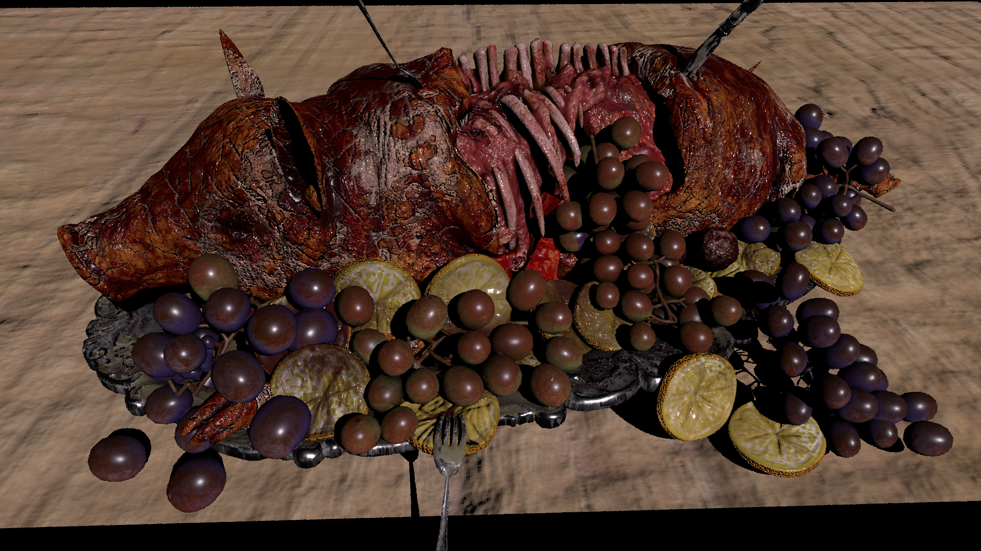
A few points about the setup.
- To isolate mip selection, I turned off stochastic effects. Secondary bounces, depth of field, and subsurface scattering are disabled. A single Dirac delta light remains. Every image is fully deterministic, which makes comparison much easier.
- Monte Carlo integration anti aliases as sample count increases. Every variant except the reference therefore uses one sample per pixel.
- In the current mip selection algorithm, when the desired level falls between N and N+1, only level N is chosen. That avoids extra blur and keeps memory use lower. The trade off is a noisier image when samples are scarce, which is acceptable in offline rendering.
A few observations from the comparison.
- Without manual mip bias, selection generally tracks the reference. It can still diverge in places, which is expected for the reasons noted earlier.
- Forcing one mip level lower sometimes works, but often introduces blur. A manual bias of +2 levels is noticeably blurrier than zero bias. Taken together, that suggests the derivatives SSL produces are a reasonable approximation of the desired signal.
- Zero bias reduces aliasing compared with −1 bias in some areas. The floor pixels show this most clearly here. In real time rendering, that kind of aliasing reduction matters. In offline rendering, higher sample counts usually mask the difference.
- We assumed each hit triangle behaves like an infinite plane, and the shaders in this asset read only
uvwfrom the SSL global to drive texture coordinates. Under those conditions, mip selection for a small triangle may appear consistent even though not strictly identical. That can in theory produce discontinuities at triangle edges, especially when there is no trilinear sampling, but in practice they are hard to see. So I’ll just leave it this way until it needs a solutioin next. Below is SORT’s mip selection debug view for this shot.
Last, let’s compare the difference of mip selection method in a final render shot, which is what we care most at the end of the day.


The result above generally matches my expectations. The regions marked by the default green square look reasonably similar to the reference image. With one extra mip level toward the coarse tier, the image turns blurry immediately, a good sign that our derivatives produce reasonable values. However, some attentive readers may also notice extra blur in the default orange region, even with the solution described in this post. That is expected. Much better results there would require anisotropic filtering, which is absent from SORT’s current prototype.
Regarding the several spots in this comparison that still show slightly blurry issue with the current solution, for example the yellow logo on the brown bag. The reason becomes immediately clear if we take a look a texture sampling at one of those pixels. Below shows the derivative coverage and mip sampling footprint of the texture.
x and y respectively. The red rectangle is the footprint of the mip level that was actually loaded.If we draw a parallelogram that just spans the derivative lines, it is much smaller than the red rectangle, so the mipped fetch covers significantly more texels than the area of interest. That gap is the root cause of the extra blur in the UV derivative image above.
The prototype picks the mip level from the maximum of the four UV partials. That is a simple rule and could likely be improved. Mip selection is largely orthogonal to the derivative propagation work in this post, so I leave that for future work.
I’m generally happy with the derivative evaluation solution now deployed in the SORT renderer despite some minor flaw. Derivative quality is hard to quantify, but much of the data above suggests that automatic differentiation produces sensible UV partials.
Conclusion
Procedural UVs in SSL broke the usual fixed function derivative pipeline, which blocked the mipmapped texture path SORT needs for a paging texture cache. The fix splits across the renderer and the compiler. SORT seeds screen space partials for each global at the hit point, and SSL propagates them through the shader graph with forward mode automatic differentiation wherever texture samples or explicit ddx / ddy calls create demand.
The benchmarks suggest the cost is manageable. Compile time can rise for shaders that need derivatives, but that work happens once at startup. Runtime overhead stayed small in the tests.
This closes a gap that has been open in SORT for years. Mipmap selection now works with arbitrary procedural texture coordinates, and the renderer has what it needs to move toward a proper texture cache without giving up shader graph flexibility.
Unfortunately, the work described in this post is not available in my public repository. Readers who want the same capability will need to implement it themselves, using this post as a guide.
Last but not least, I want to mention how heavily AI helped on this mini project. I had been stuck on this problem for years until I finally committed to it recently. I initially expected at least a year of work, since the feature touches so much of my shading language. I started using AI assisted coding only lately, and it turned out to be a strong fit. I already had a clear picture of how the pieces should fit together. AI handled much of the labor while I steered the design and broke the work into steps toward the overall goal.