I am working on material system in my renderer recently. My old implementation of microfacet models only supports isotropic BRDF, as a result of which, it can’t render something like brushed metals in my renderer. After spending three days in my spare time to extend the system to support anisotropic microfacet BRDF, I easily noticed how much mathematics that it needs to understand all the importance sampling methods. The fact that $ \theta $ and $ \phi $ are somewhat correlated makes the importance sampling a lot more complex than isotropic model. For a detailed derivation of isotropic microfacet importance sampling, please check out my previous blog. I strongly suggest checking it out if the math formula in this blog confuses you because there are a lot of basics that I won’t mention in this blog.

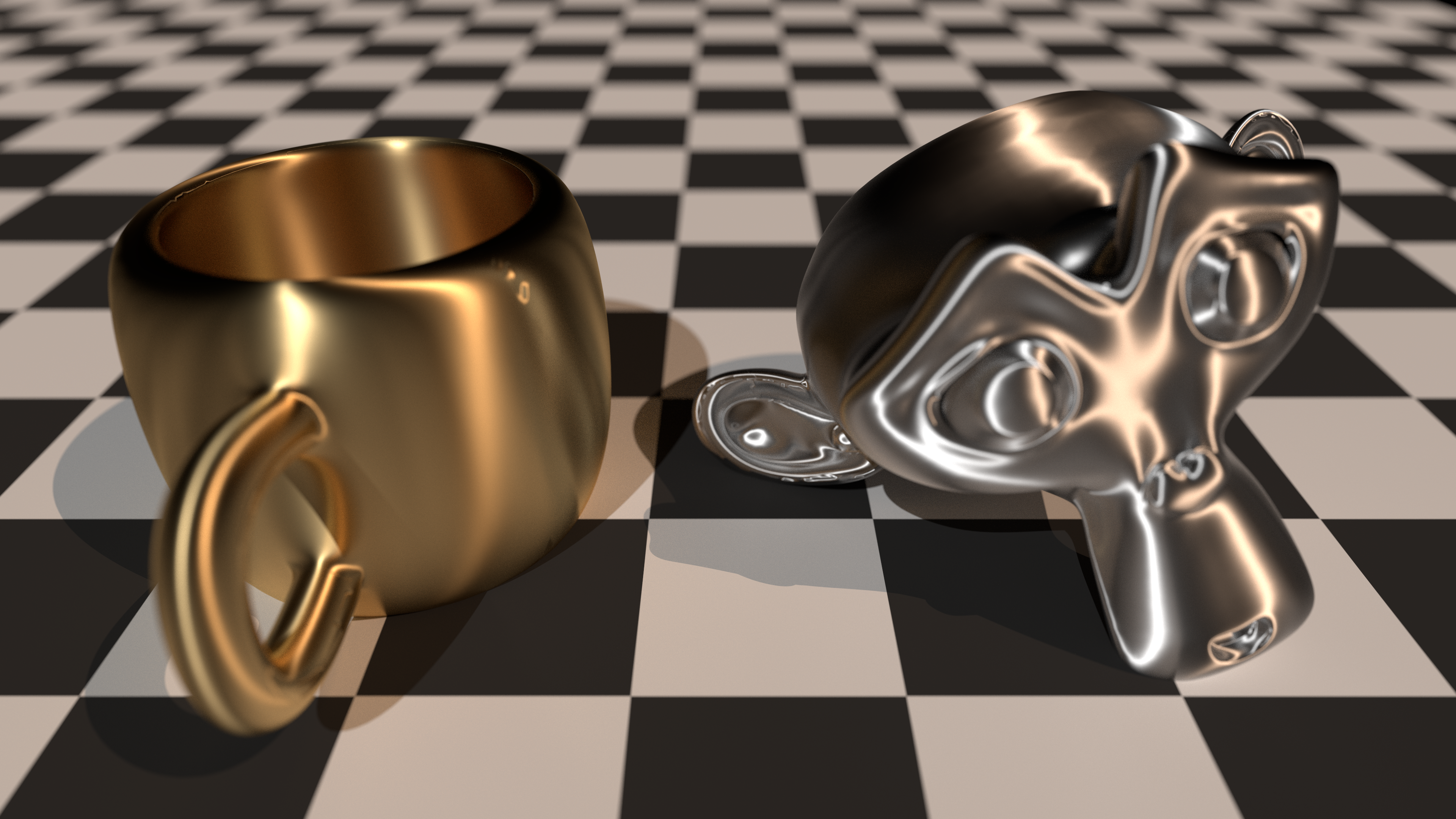
It is gonna be very boring to go through the whole blog. In case you are already bored, here is what you can achieve with the BRDF model. Hopefully, this image can convince you reading through it.

Sampling GGX

Following is the formula of GGX:

$$ D(h) = \dfrac{1}{\pi \alpha_u \alpha_v cos^4(\theta) \Big( 1 +tan^2(\theta) \Big( {\frac{cos^2(\phi)}{\alpha_u^2 }} + {\frac {sin^2(\phi) }{\alpha_v^2 }}\Big) \Big) ^ 2 } $$

Then the pdf that we choose to sample this function is:

$$ p(\theta,\phi) = \dfrac{sin(\theta)}{\pi \alpha_u \alpha_v cos^3(\theta) \Big( 1 + tan^2(\theta) \Big( {\frac{cos^2(\phi)}{\alpha_u^2 }} + {\frac {sin^2(\phi) }{\alpha_v^2 }} \Big) \Big) ^ 2 } $$

Since this is a joint density probability function of $ \phi $ and $ \theta $, we need to take one sample based on the marginal density probability function first and then take the second sample based on the conditional density function. Let’s take a look at the CDF for $ \theta $ first.

$$ P_{\theta}(\theta,\phi) = \int_0^{\theta} p(t,\phi) d(t) = \int_0^{\theta} \dfrac{sin(t)}{\pi \alpha_u \alpha_v cos^3(t) \Big( 1 + tan^2(t) \Big( {\frac{cos^2(\phi)}{\alpha_u^2 }} + {\frac {sin^2(\phi) }{\alpha_v^2 }} \Big)\Big) ^ 2 } d(t)$$

Since we are not integrating $ \phi $, I’d like to define a helper term to make the whole derivation shorter.

$$ A(\phi) = {\dfrac{cos^2(\phi)}{\alpha_u^2 }} + {\dfrac {sin^2(\phi) }{\alpha_v^2 }} $$

And then $ P_{\theta}(\theta,\phi) $ becomes this:

$ \begin{array} {lcl} P_{\theta}(\theta,\phi) &=& \int_0^{\theta} \dfrac{sin(t)}{\pi \alpha_u \alpha_v cos^3(t) ( 1 + tan^2(t) A(\phi) ) ^ 2 } d(t) \\\\ & = & \dfrac{1}{\pi \alpha_u \alpha_v} \int_0^{\theta} \dfrac{-1}{cos^3(t) ( 1 + tan^2(t) A(\phi) ) ^ 2 } d(cos(t)) \\\\ & = & \dfrac{1}{\pi \alpha_u \alpha_v} \int_0^{\theta} \dfrac{-cos(t)}{cos^4(t) ( 1 + tan^2(t) A(\phi) ) ^ 2 } d(cos(t)) \\\\ & = & \dfrac{1}{2 \pi \alpha_u \alpha_v} \int_0^{\theta} \dfrac{-1}{ ( cos^2(t) + sin^2(t) A(\phi) ) ^ 2 } d(cos^2(t))  \\\\ &= &  \dfrac{1}{2 \pi \alpha_u \alpha_v} \int_0^{\theta}  \dfrac{-1}{ ( cos^2(t) ( 1 - A(\phi) ) + A(\phi) ) ^ 2 } d(cos^2(t)) \\\\ &= &  \dfrac{1}{2 \pi \alpha_u \alpha_v ( 1 - A(\phi) ) } \int_0^{\theta} \dfrac{-1}{ ( cos^2(t) ( 1 - A(\phi) ) + A(\phi) ) ^ 2 } d( ( 1 - A(\phi) ) cos^2(t)) \\\\ &= &  \dfrac{1}{2 \pi \alpha_u \alpha_v ( 1 - A(\phi) ) } \int_0^{\theta} d \Big( \dfrac{1}{ cos^2(t) ( 1 - A(\phi) ) + A(\phi) } \Big) \\\\ &= &  \dfrac{1}{2 \pi \alpha_u \alpha_v ( 1 - A(\phi) ) } \Big( \dfrac{1}{ cos^2(\theta) ( 1 - A(\phi) ) + A(\phi) } - 1 \Big) \end{array} $

Since there is still $ \phi $ in the above CDF, we can not just use the inversion method here directly. However, this above function is gonna help us defining the marginal probability density function for $ \phi $ and conditional probability density function for $ \theta $. Following is the marginal probability density function for $ \phi $:

$$ \begin{array} {lcl} p_{\phi}(\phi) &=& \int_0^{0.5 \pi} p(\theta,\phi) d(\theta) \\\\ &=& P_{\theta}( 0.5\pi , \phi ) \\\\ &=& \dfrac{1}{2 \pi \alpha_u \alpha_v ( 1 - A(\phi) ) } \Big( \dfrac{1}{ cos^2( 0.5 \pi ) ( 1 - A(\phi) ) + A(\phi) } - 1 \Big) \\\\ &=& \dfrac{1}{2 \pi \alpha_u \alpha_v A(\phi) } \end{array}$$

By extending A in the above formula, we can easily get the marginal probability density function as following:

$ p_{\phi}(\phi) = \dfrac{1}{2 \pi \alpha_u \alpha_v \Big( {\frac{cos^2(\phi)}{\alpha_u^2}} + {\frac {sin^2(\phi) }{\alpha_v^2}} \Big) } $

Then we will use the inversion method. So the CDF of the above function is:

$$ \begin{array} {lcl}  P_{\phi}(\phi) &=& \int_{0}^{\phi} p_{\phi}(t) dt \\\\ &=& \int_{0}^{\phi} \dfrac{1}{2 \pi \alpha_u \alpha_v \Big( {\frac{cos^2(t)}{\alpha_u^2}} + {\frac {sin^2(t) }{\alpha_v^2}} \Big) } dt \\\\ &=& \dfrac{1}{2 \pi \alpha_u \alpha_v} \int_{0}^{\phi} \dfrac{1}{ cos^2(\theta) \Big( {\frac{1}{\alpha_u^2}} + {\frac {tan^2(t) }{\alpha_v^2}} \Big) } dt \\\\ &=& \dfrac{1}{2 \pi \alpha_u \alpha_v} \int_{0}^{\phi} \dfrac{1}{ {\frac{1}{\alpha_u^2}} + {\frac {tan^2(t) }{\alpha_v^2}} } d(tan(t)) \\\\ &=& \dfrac{\alpha_u}{2 \pi \alpha_v} \int_{0}^{\phi} \dfrac{1}{ 1 + \Big(\frac { \alpha_u tan(t) }{\alpha_v}\Big)^2 } d(tan(t)) \\\\ &=& \dfrac{1}{2 \pi} \int_{0}^{\phi} \dfrac{1}{ 1 + \Big(\frac { \alpha_u tan(t) }{\alpha_v}\Big)^2 } d\Big( \frac{\alpha_u tan(t)}{\alpha_v} \Big) \\\\ &=& \dfrac{1}{2 \pi} \int_{0}^{\phi} d\Big( arctan\Big( \dfrac{\alpha_u tan(t)}{\alpha_v} \Big) \Big) \\\\ &=& \dfrac{1}{2 \pi} arctan\Big( \dfrac{\alpha_u tan(\phi)}{\alpha_v} \Big) \end{array} $$

By setting a random number ranging from 0 to 1 to the CDF, we can easily acquire the following equation:

$$ \phi = arctan\Big( \dfrac{\alpha_v}{\alpha_u} tan( 2 \pi \epsilon ) \Big) $$

Before we dive into the derivation of $ \theta $, there is one minor situation to handle. Because arctan only gives you ranges between $ -\dfrac{\pi}{2}$ and $ \dfrac{\pi}{2}$, we need to remap some value to get the full range between 0 and $ 2\pi$.

Above is a graph that I generated, since our random value goes from 0 to 1, we are only interested in ranges between 0 and 1. The factor $ \dfrac{\alpha_v}{\alpha_v} $ doesn’t affect the cycle of this function, it only affects the curve shape. It is fine to sample negative values here since $ \phi $ doesn’t always need to be positive, it can be anything as long as it covers the whole range. However, one thing that we can easily notice is that the result goes from $ -\dfrac{\pi}{2}$ and $ \dfrac{\pi}{2}$ and there is even a remap once the random value is larger than 0.5. My solution is to offset each section by an offset.

$ \phi= \begin{cases} arctan\Big( \dfrac{\alpha_v}{\alpha_u} tan( 2 \pi \epsilon ) \Big) &:x\in [0,0.25] \\\\ arctan\Big( \dfrac{\alpha_v}{\alpha_u} tan( 2 \pi \epsilon ) \Big) + \pi &:x\in (0.25,0.75) \\\\ arctan\Big( \dfrac{\alpha_v}{\alpha_u} tan( 2 \pi \epsilon ) \Big) + 2\pi &:x\in [0.75,1] \end{cases} $

Extra special attention needed here to make sure the value is correctly taken in the rare case where the random value happens to be 0.25 or 0.75 so that the final curve is a continuous one. And the $ 2 \pi $ can be totally ignored since it is the cycle of cos and sin, which is our only usage for $ \phi $. However, I’d like to add it here just to keep the result in the range of [0, $ 2 \pi $ ].

Back to the derivation of $ \theta $, let’s look at the CDF of the conditional density function:

$$ \begin{array} {lcl} P_{\theta}(\theta) &=& \int_0^{\theta} \dfrac{p(t,\phi)}{p_{\phi}(\phi)} d(t) \\\\ &=& \dfrac{\int_0^{\theta} p(t,\phi) d(t)}{p_{\phi}(\phi)} \\\\ &=& \dfrac{ P_{\theta}(\theta,\phi)}{p_{\phi}(\phi)} \\\\ &=& \dfrac{\dfrac{1}{2 \pi \alpha_u \alpha_v ( 1 - A(\phi) ) } \Big( \dfrac{1}{ cos^2(\theta) ( 1 - A(\phi) ) + A(\phi) } - 1 \Big)}{\dfrac{1}{2 \pi \alpha_u \alpha_v A(\phi) }} \\\\ &=& \dfrac{A(\phi)}{ 1 - A(\phi) } \Big( \dfrac{1}{ cos^2(\theta) ( 1 - A(\phi) ) + A(\phi) } - 1 \Big) \end{array} $$

Again let’s set a random value from 0 to 1 to the CDF

$$ \begin{array} {lcl} && \epsilon = \dfrac{A(\phi)}{ 1 - A(\phi) } \Big( \dfrac{1}{ cos^2(\theta) ( 1 - A(\phi) ) + A(\phi) } - 1 \Big) \\\\ &->& \dfrac{ \epsilon ( 1 - A(\phi) ) }{ A(\phi) } + 1 = \dfrac{1}{ cos^2(\theta) ( 1 - A(\phi) ) + A(\phi) }  \\\\ &->& cos^2(\theta) ( 1 - A(\phi) ) + A(\phi) = \dfrac{A(\phi)}{ \epsilon ( 1 - A(\phi) ) + A(\phi) } \\\\ &->& cos^2(\theta) ( 1 - A(\phi) ) = \dfrac{A(\phi)}{ \epsilon ( 1 - A(\phi) ) + A(\phi) } - A(\phi) \\\\ &->& cos^2(\theta) ( 1 - A(\phi) ) = \dfrac{A(\phi) ( 1 - A(\phi) ) ( 1 - \epsilon ) }{ \epsilon ( 1 - A(\phi) ) + A(\phi) } \\\\ &->& cos^2(\theta) = \dfrac{A(\phi)( 1 - \epsilon ) }{ \epsilon ( 1 - A(\phi) ) + A(\phi) } \end{array} $$

Then we easily get the following formula for $ \theta $

$$ \theta = arccos\Big( \sqrt{ \dfrac{A(\phi)( 1 - \epsilon ) }{ \epsilon ( 1 - A(\phi) ) + A(\phi) } } \Big) $$

A little bit further from the above equation:

$$ \begin{array} {lcl} && tan^2(\theta) = \dfrac{1}{cos^2(\theta)} - 1 \\\\ &->& tan^2(\theta) = \dfrac{ \epsilon ( 1 - A(\phi) ) + A(\phi) }{ A(\phi) ( 1 - \epsilon ) } - 1 \\\\ &->& tan^2(\theta) = \dfrac{ \epsilon + A( \phi ) ( 1 - \epsilon ) }{ A(\phi) ( 1 - \epsilon ) } - 1 \\\\ &->& tan^2(\theta) = \dfrac{ \epsilon }{ A(\phi) ( 1 - \epsilon ) } \end{array} $$

Then $ \theta $ can also be calculated this way

$$ \theta = arctan\Big( \sqrt{ \dfrac{ \epsilon }{ ( 1 - \epsilon ) A(\phi) } } \Big) $$

This is exactly the same thing with the above one except that it has less steps. Before we move forward to the next one, here is the final formula for $ \theta $ and $ \phi $ for importance sampling of GGX

$$ \phi= \begin{cases} arctan\Big( \dfrac{\alpha_v}{\alpha_u} tan( 2 \pi \epsilon ) \Big) &:x\in [0,0.25] \\\\arctan\Big( \dfrac{\alpha_v}{\alpha_u} tan( 2 \pi \epsilon ) \Big) + \pi &:x\in (0.25,0.75) \\\\arctan\Big( \dfrac{\alpha_v}{\alpha_u} tan( 2 \pi \epsilon ) \Big) + 2\pi &:x\in [0.75,1] \end{cases} $$ $$ \theta = arctan\bigg( \sqrt{ \dfrac{ \epsilon }{ ( 1 - \epsilon ) \Big({\dfrac{cos^2(\phi)}{\alpha_u^2 }} + {\dfrac {sin^2(\phi) }{\alpha_v^2 }}\Big)} } \bigg) $$

Sampling Beckmann

Several concepts are very similar to the above derivation, which we will skip here for simplicity.

The formula for Beckmann is as following:

$$ D(h) = \dfrac{ e^{-tan^2(\theta)\Big( (\frac{cos(\phi)}{\alpha_u})^2 + (\frac{sin(\phi)}{\alpha_v})^2 \Big) } }{\pi \alpha_u \alpha_v cos^4(\theta) } $$

As usual, the PDF that we use to sample Beckmann is defined as following:

$$ p(\theta,\phi) = \dfrac{ sin(\theta) \Bigg(e^{-tan^2(\theta)\Big( (\frac{cos(\phi)}{\alpha_u})^2 + (\frac{sin(\phi)}{\alpha_v})^2 \Big) } \Bigg)}{\pi \alpha_u \alpha_v cos^3(\theta) } $$

Let’s look at the CDF for $ \theta $:

$$ P_{\theta}(\theta,\phi) = \int_0^{\theta} p(t,\phi) d(t) = \int_0^{\theta} \dfrac{ sin(t) \bigg(e^{-tan^2(t)\Big( (\frac{cos(\phi)}{\alpha_u})^2 + (\frac{sin(\phi)}{\alpha_v})^2 \Big) } \bigg)}{\pi \alpha_u \alpha_v cos^3(t) } d(t) $$

We gonna use the same A term that we defined earlier to simplify the derivation:

$$ \begin{array} {lcl} P_{\theta}(\theta,\phi) &=& \int_0^{\theta} \dfrac{ sin(t) (e^{-tan^2(t) A(\phi) } )}{\pi \alpha_u \alpha_v cos^3(t) } d(t) \\\\ &=& \dfrac{-1}{\pi \alpha_u \alpha_v} \int_0^{\theta} \dfrac{ e^{-tan^2(t) A(\phi) } }{ cos^3(t) } d(cos(t)) \\\\ &=& \dfrac{1}{2 \pi \alpha_u \alpha_v} \int_0^{\theta} e^{-tan^2(t) A(\phi) } d\Big(\dfrac{1}{cos^2(t)}\Big) \\\\ &=& \dfrac{1}{2 \pi \alpha_u \alpha_v} \int_0^{\theta} e^{ \Big( 1 - \frac{1}{cos^2(t)} \Big) A(\phi) } d\Big(\dfrac{1}{cos^2(t)}\Big) \\\\ &=& \dfrac{1}{2 \pi \alpha_u \alpha_v A(\phi) } \int_0^{\theta} e^{ A(\phi) - \frac{A(\phi)}{cos^2(t)} } d\Big(\dfrac{A(\phi)}{cos^2(t)}\Big) \\\\ &=& \dfrac{-1}{2 \pi \alpha_u \alpha_v A(\phi) } \int_0^{\theta} d\Big(e^{ A(\phi) - \frac{A(\phi)}{cos^2(t)} } \Big) \\\\ &=& \dfrac{1}{2 \pi \alpha_u \alpha_v A(\phi) } \Big( 1 - e^{ A(\phi) - \frac{A(\phi)}{cos^2(\theta)} } \Big) \end{array}$$

Following is the marginal probability density function for $ \phi $

$$ \begin{array} {lcl} p_{\phi}(\phi) &=& \lim_{\theta \to {0.5\pi}} \int_0^{\theta} p(\theta,\phi) d(\theta) \\\\ &=& \lim_{\theta \to {0.5\pi}} P_{\theta}( \theta , \phi ) \\\\ &=& \lim_{\theta \to {0.5\pi}} \Big( \dfrac{1}{2 \pi \alpha_u \alpha_v A(\phi) } \Big( 1 - e^{ A(\phi) - \frac{A(\phi)}{cos^2(\theta)} } \Big) \Big) \\\\ &=& \dfrac{1}{2 \pi \alpha_u \alpha_v A(\phi) } \end{array}$$

One minor detail to notice is that since we can’t really approach 90 degree angle for $ \theta $, we will not take it into consideration here. Surprisingly, this is exactly the same with GGX’s marginal probability density function, so we will take everything we have derived here to avoid the duplicated work so that we can move forward to the CDF for $ \theta $ directly

$$ \begin{array} {lcl} P_{\theta}(\theta) &=& \int_0^{\theta} \dfrac{p(t,\phi)}{p_{\phi}(\phi)} d(t) \\\\ &=& \dfrac{\int_0^{\theta} p(t,\phi) d(t)}{p_{\phi}(\phi)} \\\\ &=& \dfrac{ P_{\theta}(\theta,\phi)}{p_{\phi}(\phi)} \\\\ &=& \dfrac{\frac{1}{2 \pi \alpha_u \alpha_v A(\phi) } \Big( 1 - e^{ A(\phi) - \frac{A(\phi)}{cos^2(\theta)} }\Big)}{ \frac{1}{2 \pi \alpha_u \alpha_v A(\phi) }} \\\\ &=&  1 - e^{ A(\phi) - \frac{A(\phi)}{cos^2(\theta)} } \\\\ &=&  1 - e^{ - A(\phi) tan^2(\theta) } \end{array} $$

By setting the CDF to $ \epsilon $ it is not hard to get the following equation:

$$ \theta = arctan\Bigg( \dfrac{ln(1-\epsilon)}{A(\phi)} \Bigg) = arctan\Bigg( \dfrac{ln(1-\epsilon)}{{\frac{cos^2(\phi)}{\alpha_u^2 }} + {\frac {sin^2(\phi) }{\alpha_v^2 }}} \Bigg) $$

Since $ \epsilon $ is randomly chosen between 0 and 1, we can easily replace $ 1 - \epsilon $ with $ \epsilon $ itself, resulting in the final formula for $ \theta $

$$ \theta = arctan\Bigg( \dfrac{ln(\epsilon)}{{\frac{cos^2(\phi)}{\alpha_u^2 }} + {\frac {sin^2(\phi) }{\alpha_v^2 }}} \Bigg) $$

To summarize, following are the formula we used to importance sample Beckmann:

$$ \phi= \begin{cases} arctan\Big( \dfrac{\alpha_v}{\alpha_u} tan( 2 \pi \epsilon ) \Big) &:x\in [0,0.25] \\\\arctan\Big( \dfrac{\alpha_v}{\alpha_u} tan( 2 \pi \epsilon ) \Big) + \pi &:x\in (0.25,0.75) \\\\arctan\Big( \dfrac{\alpha_v}{\alpha_u} tan( 2 \pi \epsilon ) \Big) + 2\pi &:x\in [0.75,1] \end{cases} $$ $$ \theta = arctan\Bigg( \dfrac{ln(\epsilon)}{{\frac{cos^2(\phi)}{\alpha_u^2 }} + {\frac {sin^2(\phi) }{\alpha_v^2 }}} \Bigg) $$

Sampling Blinn

Here we will talk about the modified Blinn-Phong model, instead of the original one proposed in paper ( An Anisotropic Phong BRDF Model ), because it obeys the rule of energy conservation. And the other detail that deserves mentioning is that I will use the exponent term instead of alpha term here:

$$ e = \dfrac{2.0}{\alpha^4} - 2.0 $$

It goes true along both directions. And the evaluation of Blinn is as following:

$$ D(h) = \dfrac{\sqrt{( e_u + 2 ) * ( e_v + 2 ) }}{2\pi} cos(\theta) ^ {( cos^2(\phi) * e_u + sin^2(\phi) * e_v ) } $$

Following is the pdf we use to sample Blinn:

$$ p( \theta , \phi ) = \dfrac{\sqrt{( e_u + 2 ) * ( e_v + 2 ) }}{2\pi} sin(\theta ) cos(\theta) ^ {( cos^2(\phi) * e_u + sin^2(\phi) * e_v + 1 ) } $$

The CDF for $ \theta $ is as following:

$$ P_{\theta}(\theta,\phi) = \int_0^{\theta} p(t,\phi) d(t) = \int_0^{\theta} \dfrac{\sqrt{( e_u + 2 ) * ( e_v + 2 ) }}{2\pi} sin(t) cos(t) ^ {( cos^2(\phi) * e_u + sin^2(\phi) * e_v + 1 ) } dt $$

Before we move forward, let’s define a B term to make the whole derivation shorter:

$$ B(\phi) = cos^2(\phi) * e_u + sin^2(\phi) * e_v $$

And then the above formula becomes:

$$ \begin{array} {lcl} P_{\theta}(\theta,\phi) &=& \int_0^{\theta} \dfrac{\sqrt{( e_u + 2 ) * ( e_v + 2 ) }}{2\pi} ( cos(t) ^ {( B(\phi) + 1 ) } ) sin(t) dt \\\\ &=& \dfrac{-\sqrt{( e_u + 2 ) * ( e_v + 2 ) }}{2\pi} \int_0^{\theta} cos(t) ^ {( B(\phi) + 1 ) } d( cos(t) ) \\\\ &=& \dfrac{-\sqrt{( e_u + 2 ) * ( e_v + 2 ) }}{ 2\pi ( B(\phi) + 2 ) } \int_0^{\theta} d( cos(t) ^ { {B(\phi) + 2 }} ) \\\\ &=& \dfrac{\sqrt{( e_u + 2 ) * ( e_v + 2 ) }}{2 \pi ( B(\phi) + 2 ) } ( 1 - cos(\theta) ^ {( B(\phi) + 2 ) } ) \end{array}$$

Following is the marginal probability density function for $ \phi $:

$$ \begin{array} {lcl} p_{\phi}(\phi) &=& \int_0^{0.5 \pi} p(\theta,\phi) d(\theta) \\\\ &=& P_{\theta}( 0.5\pi , \phi ) \\\\ &=& \dfrac{\sqrt{( e_u + 2 ) * ( e_v + 2 ) }}{ 2\pi ( B(\phi) + 2 ) } ( 1 - cos( 0.5 \pi ) ^ {( B(\phi) + 2 ) } ) \\\\ &=& \dfrac{\sqrt{( e_u + 2 ) * ( e_v + 2 ) }}{ 2 \pi ( B(\phi) + 2 ) } \\\\ &=& \dfrac{\sqrt{( e_u + 2 ) * ( e_v + 2 ) }}{ 2 \pi ( cos^2(\phi) * e_u + sin^2(\phi) * e_v + 2 ) } \end{array}$$

The CDF for $ \phi $ is:

$$ \begin{array} {lcl} P_{\phi}(\phi) &=& \int_0^{\phi} p_{\phi}(t) d(t) \\\\ &=& \int_0^{\phi}\dfrac{\sqrt{( e_u + 2 ) * ( e_v + 2 ) }}{ 2 \pi ( cos^2(t) * e_u + sin^2(t) * e_v + 2 ) } d(t) \\\\ &=& \dfrac{\sqrt{( e_u + 2 ) * ( e_v + 2 ) }}{2\pi} \int_0^{\phi}\dfrac{1}{ cos^2(t) * e_u + sin^2(t) * e_v + 2 ( cos^2(t) + sin^2(t) ) } d(t) \\\\ &=& \dfrac{\sqrt{( e_u + 2 ) * ( e_v + 2 ) }}{2\pi} \int_0^{\phi}\dfrac{1}{  cos^2(t) ( e_u + 2 + tan^2(t) * ( e_v + 2 ) ) } d(t) \\\\ &=& \dfrac{1}{2\pi} \sqrt{\dfrac{ e_v + 2 }{ e_u + 2 }} \int_0^{\phi}\dfrac{1}{  1 + \Big(\sqrt{\frac{ e_v + 2 }{ e_u + 2 }} tan(t) \Big) ^ 2 } d( tan(t) ) \\\\ &=& \dfrac{1}{2\pi} \int_0^{\phi}\dfrac{1}{  1 + \Big( \sqrt{\frac{ e_v + 2 }{ e_u + 2 }} tan(t) \Big) ^ 2 } d\Big( \sqrt{\frac{ e_v + 2 }{ e_u + 2 }} tan(t) \Big) \\\\ &=& \dfrac{1}{2\pi} arctan\Big( \sqrt{\frac{ e_v + 2 }{ e_u + 2 }} tan(t) \Big) \end{array} $$

It is not hard to get the following formula for $ \phi $

$$ \phi = arctan\Big( \sqrt{\dfrac{ e_u + 2 }{ e_v + 2 }} tan(2 \pi \epsilon) \Big) $$

And we also need to offset this parameter like we did for the previous two sampling method, but the way we do it is almost identical. Last, we need to generate $ \theta $ based on the conditional probability density function:

$$ \begin{array} {lcl} P_{\theta}(\theta) &=& \int_0^{\theta} \dfrac{p(t,\phi)}{p_{\phi}(\phi)} d(t) \\\\ &=& \dfrac{\int_0^{\theta} p(t,\phi) d(t)}{p_{\phi}(\phi)} \\\\ &=& \dfrac{ P_{\theta}(\theta,\phi)}{p_{\phi}(\phi)} \\\\ &=& \dfrac{\dfrac{\sqrt{( e_u + 2 ) * ( e_v + 2 ) }}{2 \pi ( B(\phi) + 2 ) } ( 1 - cos(\theta) ^ {( B(\phi) + 2 ) } )}{\dfrac{\sqrt{( e_u + 2 ) * ( e_v + 2 ) }}{ 2 \pi ( B(\phi) + 2 ) }} \\\\ &=& 1 - cos(\theta) ^ { B(\phi) + 2 } \end{array} $$

With a random variable equals to the above CDF, we can easily have the following formula:

$$ \theta = arccos\Big( ( 1 - \epsilon ) ^ { \small \dfrac{1}{cos^2(\phi) * e_u + sin^2(\phi) * e_v + 2} } \Big) $$

And again, we can also flip the $ \epsilon $ because it goes from 0 to 1.

$$ \theta = arccos\Big( \epsilon ^ { \small \dfrac{1}{cos^2(\phi) * e_u + sin^2(\phi) * e_v + 2} } \Big) $$

Before we sumarize, here is the final formula for importance sampling of Blinn:

$$ \phi= \begin{cases} arctan\Big( \sqrt{\dfrac{ e_u + 2 }{ e_v + 2 }} tan(2 \pi \epsilon) \Big) &:x\in [0,0.25] \\\\arctan\Big( \sqrt{\dfrac{ e_u + 2 }{ e_v + 2 }} tan(2 \pi \epsilon) \Big) + \pi &:x\in (0.25,0.75) \\\\arctan\Big( \sqrt{\dfrac{ e_u + 2 }{ e_v + 2 }} tan(2 \pi \epsilon) \Big) + 2\pi &:x\in [0.75,1] \end{cases} $$ $$ \theta = arccos\Big( \epsilon ^ { \small \dfrac{1}{cos^2(\phi) * e_u + sin^2(\phi) * e_v + 2} } \Big) $$

Summary

Importance sampling is always importance for a ray tracer. With the above method, a ray tracer should be able to reach relative noise-free image with reasonalely enough sample taken per pixel.

There is also some future work improving the efficiency of importance sampling for the microfacet model, like sampling visible normal. And it is also the default method for PBRT microfacet model sampling.

If someone is interested in the detailed implementation, they can check it out in my github project here .

Reference:

[1] Marginal probability density function
[2] Conditional probability distribution
[3] Physically Based Rendering
[4] Importance Sampling Microfacet-Based BSDFs using the Distribution of Visible Normals
[5] An Improved Visible Normal Sampling Routine for the Beckmann Distribution 
[6] Specular BRDF Reference
[7] An Anisotropic Phong BRDF Model
[8] Microfacet BRDF
[9] Phong Normalization Factor derivation
[10] Sampling Microfacet BRDF