Recently, I had the pleasure of contributing to Nvidia’s Zorah project, the flagship demo for the RTX 50 Series GPUs. My primary role was to provide technical support for light transport in Zorah, which included collaborating with my colleague Daqi Lin to implement a brand new ReSTIR-based global illumination solution, specifically, ReSTIR PT^[1], within the NvRTX branch of Unreal Engine.

A GDC presentation video on Zorah was released a few weeks ago. If it slipped past your radar, here it is for your convenience.

Hopefully, this video will spark some interest and motivate readers to dive into this lengthy post. All light bounces shown in the demo are dynamically evaluated in real time. Even though I had been working on this project for months, I was still blown away when I saw it in action for the first time. It was a powerful reminder of the advancements in real-time path traced global illumination technology.

A heads-up before moving forward: technical details related to the engineering aspects of the Zorah project will not be covered in this blog post. This post actually has nothing to do with the Zorah project itself. Instead, it’s focused on explaining the theory behind ReSTIR GI^[2], rather than the engineering challenges we faced in Zorah or the theory behind ReSTIR PT. Since our ReSTIR PT implementation is built on top of an existing ReSTIR GI implementation^[3] on NvRTX branch, running ReSTIR GI in the scenes shown above would already produce an indirect diffuse GI signal that’s on par with ReSTIR PT. The main improvement introduced in ReSTIR PT is mirror reflection.

So yes, showing the video here is a bit of a cheat, as it isn’t strictly about ReSTIR GI. But it’s still by far the best visual I can share to demonstrate what ReSTIR GI is capable of when focusing solely on diffuse GI. That’s why I feel it makes sense to include it here.

For readers interested in the engineering side of the implementation, we have a GDC presentation^[4] available online, where we go into detail about how we approached the solution in Zorah. Alternatively, you can check out the open-source code in the nvrtx-5.4 branch.

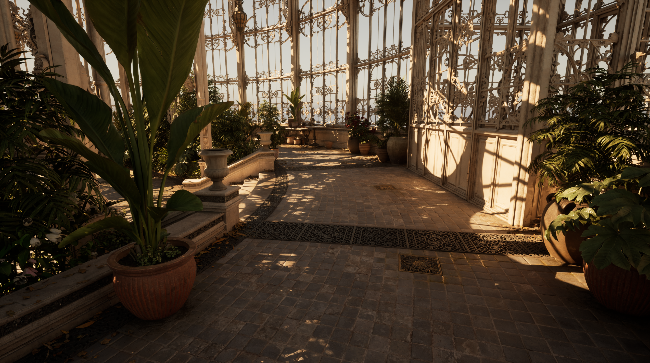
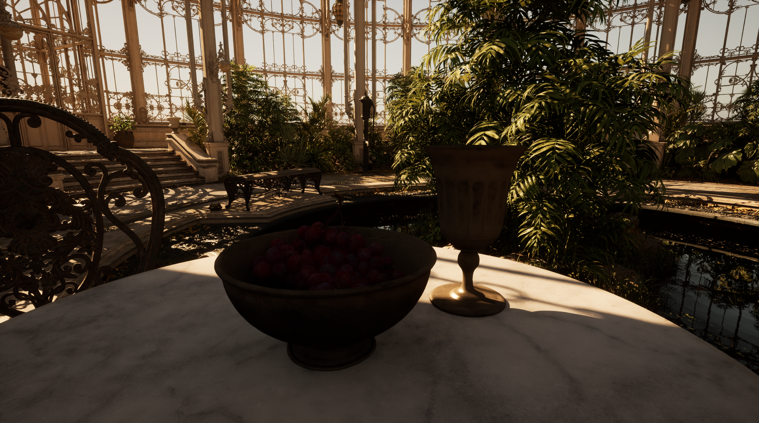
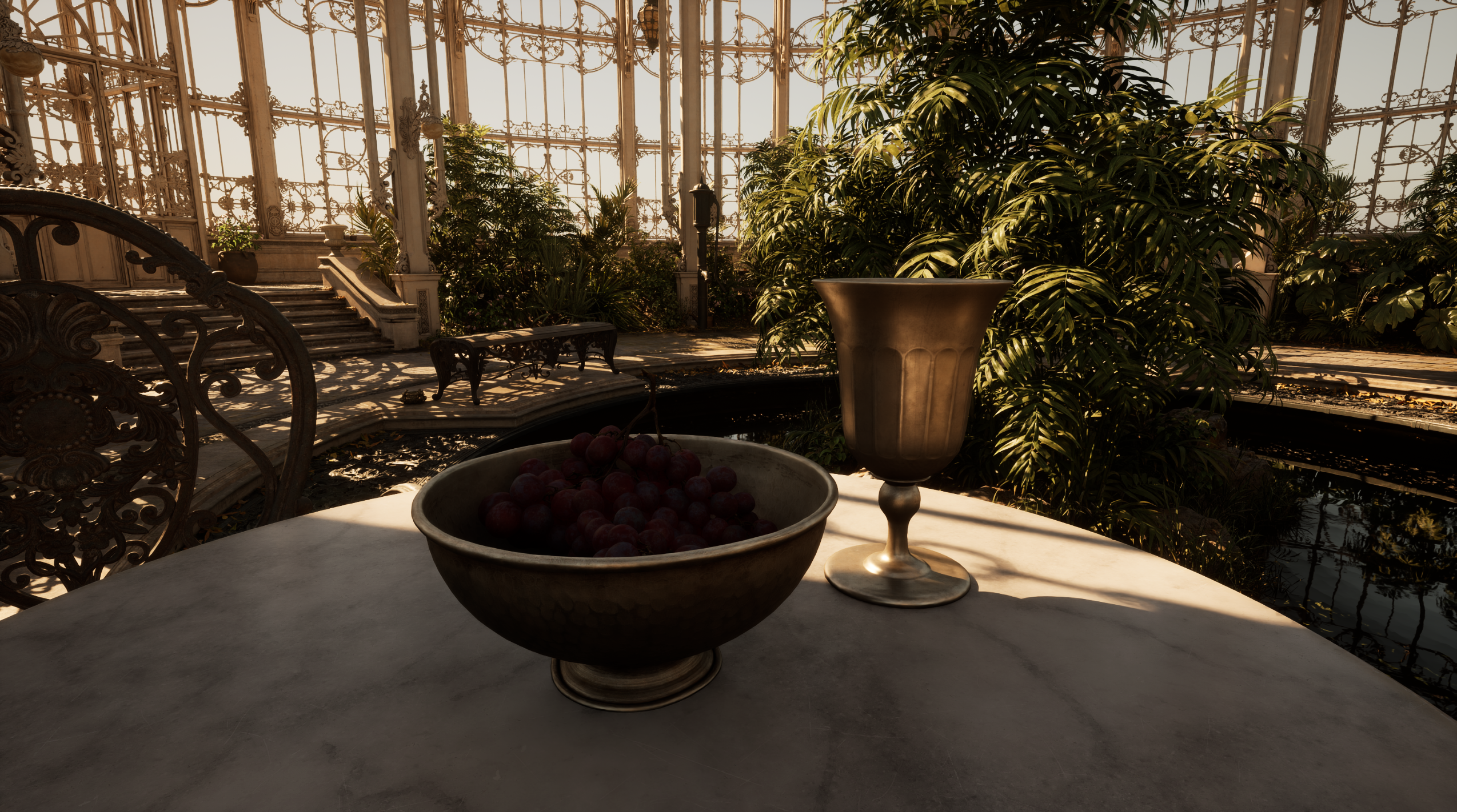
Below is a screenshot captured from one of our levels, the Greenhouse level. The GI signal is produced by ReSTIR GI, rather than ReSTIR PT. If you’re interested in trying it out yourself, here is the link for download. You’ll also need the NvRTX Experimental Branch to run this demo, as it’s required to enable Megageo (the ray tracing Nanite feature).

Introduction

About two and a half years ago, I shared a blog post^[5] discussing the fundamental mathematical theory behind ReSTIR DI^[6]. It aimed to explain the core theory behind the ReSTIR DI algorithm, the simplest form of ReSTIR. As I continued exploring various variants of this sampling approach, I gained deeper insights into how ReSTIR works. In this blog post, I’d like to share some of my thoughts in the hope of shedding light on some of the more subtle aspects of ReSTIR GI, a variant of ReSTIR designed to tackle the global illumination problem, rather than the many-light problem.

It’s important to read the original ReSTIR GI paper first, as this post won’t explain how the algorithm works. Instead, it focuses on a few mathematical aspects that can be confusing if not carefully thought through. Readers are also strongly encouraged to review the mathematical foundation of ReSTIR beforehand, as the content here may be quite confusing otherwise. Without a solid understanding of how ReSTIR works in general, it may be difficult to fully grasp the math discussed in this post.

Preliminary Reading

Similar to my previous post, let’s first go through some preliminary knowledge that is essential for understanding the math behind ReSTIR GI before diving into the explanation.

Rendering Equation

As global illumination is a more complicated topic than direct illumination, let’s start with rendering equation since we are talking about GI this time.

Strictly speaking, game engines split the rendering equation into several categories, such as emissive surfaces, direct illumination, indirect diffuse illumination, indirect smooth specular illumination, indirect rough specular illumination. It is worth noting that game engines may also have their own split based on light types as well. For example, direct illumination contribution from sky light can be evaluated in Unreal Engine’s Lumen GI system^[7]. But for simplicity, we assume this is split into three parts as it is sufficient for our discussion in this post.

• Emissive surfaces that are directly visible in primary view
• Direct illumination
• Global illumination

Let’s simply make the split here so that we are more clear about what exactly our problem set is when we talk about ReSTIR GI. Here we assume $x$ is the primary visible vertex.

Emissive surfaces are pretty easy to understand, it is area light sources (including sky light) that we can see directly in primary view. Throughout this whole blog post, we will make an assumption that the evaluation of light radiance given a light sample is deterministic and can be done in O(1) time, which is largely true in most game engines. Such a signal can simply be represented by $L_e(x, w_o)$. As we can easily notice from this form, with the above assumption, this is not even an integral estimation. There is no Monte Carlo approximation going on in real time emissive signal evaluation, hence this process will produce zero noise and commonly is not a major technical challenge in game rendering.

For our convenience, let’s define the non-emissive term explicitly. The subscript $l$ stands for light here, which is not super precise, but it is ok since we just need a term to identify the rendering equation’s integral part.

Regarding direct illumination, below is the equation for it.

This starts getting more interesting as some of the light sources, such as area light or sky light, may introduce Monte Carlo approximation. This is to support both soft shadow and the overall contribution of light sources towards a specific shading point. As long as the light source is not a Dirac delta function, this dimensionality of integral will need Monte Carlo approximation, which commonly means efficient sampling approach is needed to suppress noise to an acceptable level. And ReSTIR DI is specifically designed for it.

For the global illumination problem, below is the correct form of its math representation.

Things get a lot more complicated here. It all starts from the fact that $L_l$ doesn’t have a closed form solution in most cases, unlike $L_e$ which we assume can be evaluated in O(1) time in deterministic manner. Or put it another way, this equation requires higher dimensional integral than the DI integral. As a matter of fact, this equation is an integral of infinite dimensions. Clearly, the GI problem is a much more complicated problem compared with DI, which largely thanks to the $L_l(w_i)$ lacks a deterministic evaluation. The truth is approximating $L_l(w_i)$ is equally challenging as solving the rendering equation in the first place as it expands to a rendering equation without the emissive term.

With such a complicated problem, native sampling approach based on BRDF PDF for drawing continuation ray with NEE samples may lose its efficiency in some cases. Algorithms like path guiding ^{[8, 9]} are designed for improved sampling efficiecny. Unlike path guiding, without requiring complex data structure, ReSTIR GI also aims to effectively improve the sampling efficiency for equation 4.

Primary Sample Space

Primary sample space, or PSS for short, is critical for us to understand ReSTIR GI, later we will see its application in it. To understand how it works in a path tracer, readers can take a look at the S3 section of GRIS paper’s supplementary material^[1].

For your convenience, I’d also like to put down some explaination here. Different from the supplemental material, I’d like to explain PSS without assuming any graphics context. Imagine we are estimating the following integral with Monte Carlo method.

This is pretty basic. Here are the common steps to approximate it with Monte Carlo method.

1. Produce a random number $u_i$ that is uniformly distributed between 0 and 1
2. Draw a sample $x_i$ with some sampling PDF with the the random number $u_i$
3. Throw this sample $x_i$ in $f(x)$ and accumulate a sum with $f(x_i)/p_x(x_i)$
4. Go back to step 1 until we hit here N times
5. Divide the accumulted result by N

The Monte Carlo estimator for this integral is simply this

I added a subscript $x$ for $p(x)$ just to indicate samples are drawn in $x$’s domain. The same goes true for all $x_i$ within $\hat{I}_N$, which means it is an estimator based on drawing samples in $x$’s domain.

The whole sampling process starts with a uniformly distributed random number between 0 and 1. We can actually see $x$ as a function of $u$, which is essentially what it is. With this mental shift, we can rewrite the above estimator this way under the condition that each $u$ only maps to a unique $x$

I’d like to bring up another fact here that the PDF for $u$ is simply 1. Or put it in simple math

Combine equation 7 and equation 8, we can rewrite equation 7 this way

This looks unnecessarily complicated given that we haven’t changed anything for real. But now, let’s put estimator 9 on hold for a short while and try to Monte Carlo sample the integral below next.

Don’t be intimidated by $\dfrac{f(x(u))}{p_x(x(u))}$, you can simply regard it as a new function of $u$. And this $\Omega_u$ is essentially is a high dimensional cube. Applying the same steps mentioned above, except this time our samples are merely random numbers from 0 to 1, we have this Monte Carlo estimator for this integral.

Taking one step back, this happens to be exactly the same thing as estimator 9, which is what we can use to approximate the integral 5. Now we can see, with one single estimator, we can approximate the value of two seemingly different integrals in an unbiased and consistent manner. This safely gives us a simple conclusion.

Putting it in another way, in order to approximate the integral over $x$’s domain for $f(x)$, we can simply integrate over a high dimensional (equal dimension with $x$) unit cube domain and use the latter integral (integral 10) instead as long as we have a PDF method in our mind that we can use to draw sample $x$ from.

In case anyone is still curious why this can magically happen, the following derivation will uncover the mystery.

If anyone has trouble in figuring out how $p_x(x(u))$ is converted to $p_u(u) / |x’(u)|$, please check this chapter in pbrt^[10]. I won’t put down that simple derivation here to save some text.

The above derivation works with both scalar inputs and vector inputs, both $x$ and $u$ can be a multi-dimentional input, rather than a scalar. With vectors as inputs, the first way we prove PSS doesn’t change at all, while we need to swap the derivation $f’(x)$ by Jacobian in second proof in derivation 13.

Per Initial Candidate Target Function in RIS

Resampled importance sampling is a sampling method to draw higher quality samples based on a bunch of lower quality candidate samples drawn from proposal PDFs^[11]. It provides an unbiased Monte Carlo approximation of an integral by approximating generating samples based on some target function distribution, which doesn’t have to be normalized. Its realized PDF is intractable, but we know it approaches to normalized target function with growing number of proposal candidates. Let’s briefly go over how RIS works.

To approximate the integral of $f(x)$ over a specific domain, here is what we need to do with RIS

• Produces a bunch of proposal candidates $x_i$ based on some proposal PDF. We could draw proposal candidates from multiple different proposal PDFs, rather than just one.
• Define a target function $\hat{p}(x_i)$, which ideally should match the integrand well. A constant scaling factor on the target function shouldn’t matter, meaning this target function doesn’t have to be normalized.
• For each proposal candidate, we assign a resampling weight, which is $w_i(x_i) = m_i(x_i) \hat{p}(x_i) / p_i(x_i) $. Here, $m_i(x_i)$ is the MIS weight^[12].
• Draw a sample by streaming in the proposal candidates. Each proposal candidate can be chosen based on their resampling weight. Specifically, the probablity of them being chosen is proportional to the resampling weight. This process is commonly done through an algorithm called weighted reservoir sampling^[13].
• The unbiased approximation of the reciprocal of the PDF producing this final sample is the combined resampling weights of visited proposal candidates divided by the target function value evaluated at the chosen sample. This is called unbiased contribution weight^[14], UCW for short.

At this point, with the unbiased contribution weight, we should be able to throw the RIS sample in a Monte Carlo estimator for approximating the integral.

The GRIS paper provides a fairly in-depth analysis of how to generalize RIS^[1]. The paper points it out that proposal candidates drawn from different proposal PDFs don’t have to be in the same domain. It could be in different domains. Upon resampling, we should apply a shift mapping to convert the sample to the current domain of our interest and a Jacobian to the proposal PDF or UCW. Essentially, this is the theoritical foundation for ReSTIR GI as well, except that this GRIS idea was not published by the time ReSTIR GI paper was out. We can treat ReSTIR GI as one use case of GRIS theory. Without introducing the complexity in this post, I will try explaining how this is done without going through the details in this GRIS paper in the following section. However, readers are strongly recommended to go through it^[1] and the Siggraph course^[14] to gain a deeper understanding of this.

Our interest in this section is about target function. After some careful derivation, it turns out that a different target function can be applied to each initial candidate. To clarify, the choice of using a different or the same target function is completely independent of whether the proposal candidates are drawn from the same proposal PDF or not. It is rarely mentioned in most sources that target function can be per proposal candidate, which gives us an impression that target function has to be the same for RIS process. And this is certainly not true. In order to prove so, let’s define resampling weight with the revised version as below.

To be clear, $y$ is the chosen sample and $s$ is the index of the chosen sample. Please be mindful that in the above equation 14, we put a subscript at $\hat{p}_i$ to indicate it is per candidate now. This means we now allow different target functions to be applied during RIS. Below is the derivation of the revised algorithm.

The whole derivation still stands even if there is a different target function for each proposal candidate. This may sound useless at the beginning as we won’t know what the RIS sample PDF will converge to. But not having the restriction that we have to use a same target function throughout the whole process is certainly a welcome flexibility. In my previous blog post^[5], I explained in detail in a section visibility reuse why mixing target function with and without visibility check could be valid in ReSTIR DI. Back then, I didn’t realize target function has this flexibility. With the above derivation, a much easier way to explain it is we simply can do so thanks to the per initial candidate target function flexibility allowed in RIS.

ReSTIR GI Details

A typical structure of ReSTIR implementation looks like this

This goes true for both ReSTIR DI and ReSTIR GI. Please be mindful that sometimes for performance reason, initial sampling and temporal resampling pass may be fused together to save some bandwidth cost. But the general logical structure remains the same.

ReSTIR, as its name implies, is a combination of temporal and spatial resampling algorithm. Without strict definition, the common sense is initial sampling pass is also part of ReSTIR. There is a decent amount of content in the original ReSTIR DI paper that is about how to apply RIS in the initial sampling pass. In ReSTIR PT, it needs to resample one single path from a path tree in the initial sampling pass for it to work. (A path tree is the union of all paths of different depth produced by a single sample)

On a side note, we can apply this structure to lots of other sampling problems as long as there is some form of coherence, in the case of ReSTIR GI it is temporal coherence between frames and spatial coherence between pixels on screen. The problem to be sampled doesn’t need to be graphics relevant. To some degree, ReSTIR is essentially a generic importance sampling algorithm that helps produce high quality samples for Monte Carlo method.

We commonly see the green passes as the core of ReSTIR. The general structure of ReSTIR is fairly similar between ReSTIR DI and ReSTIR GI. Even the implementation of ReSTIR (temporal + spatial) is largely similar. As we can see, the exact problem ReSTIR solves heavily depends on what the concept of initial candidate is in the initial sampling pass and what integral we try to approximate in the final evaluation pass. Clearly, the concept of initial candidate and final integrand has to match to make sense.

In ReSTIR DI, it is fairly simple and clear what initial candidate is. It is nothing but a sample (point) on light sources. And the integral is simply integral 3. W.r.t ReSTIR GI, the problem set seems to be integral 4 and I also mention initial candidate is a path tree in my presentation^[4], which is not wrong, but not very precise either. I had to explain it that way due to time limitation in our talk. There was certainly not enough time in our sharing for me to go through the math that we will mention in this blog post next. Hopefully, the following explanation in this post will fill in the gap. Understanding these details is the key to get ReSTIR GI implemented done right.

Initial Candidates in ReSTIR GI

There are a few items needed to be cleared before we put our hands on an actual implementation of ReSTIR GI.

• What exactly is the problem we are trying to solve
• What target function should we use to weight samples during resampling
• What is the precise definition of initial candidate concept
• What is the proposal PDF of producing this initial candidate

The least interesting topic is the second one, there are two mentioned in the paper, one of which is the radiance from $x_2$ (secondary bounce) to $x_1$ (primary bounce), the other one is simply $L_l(\omega_{i}) f( x_1, \omega_{i}, \omega_{o} ) cos(\theta_{i})$. As a matter of fact, choice of target function, as long as it meets certain condition, won’t have impact on the unbiasness of the approximation, though they will indeed have impact on how fast the approximation converges. Even though we will not primarily focus on this topic in the following sections, we will still revise this later to be more precise.

A Possible Solution?

Our particular interest are the other three items. At the end of last section, we mentioned that the problem could be integral 4. The initial candidate could be a path tree, which is defined as the combination of paths of all depth as mentioned earlier. And to be clear, our path tree concept excludes DI path since it is not part of ReSTIR GI. This seemingly well-made decision will not work well once we consider the proposal PDF of producing the path tree next.

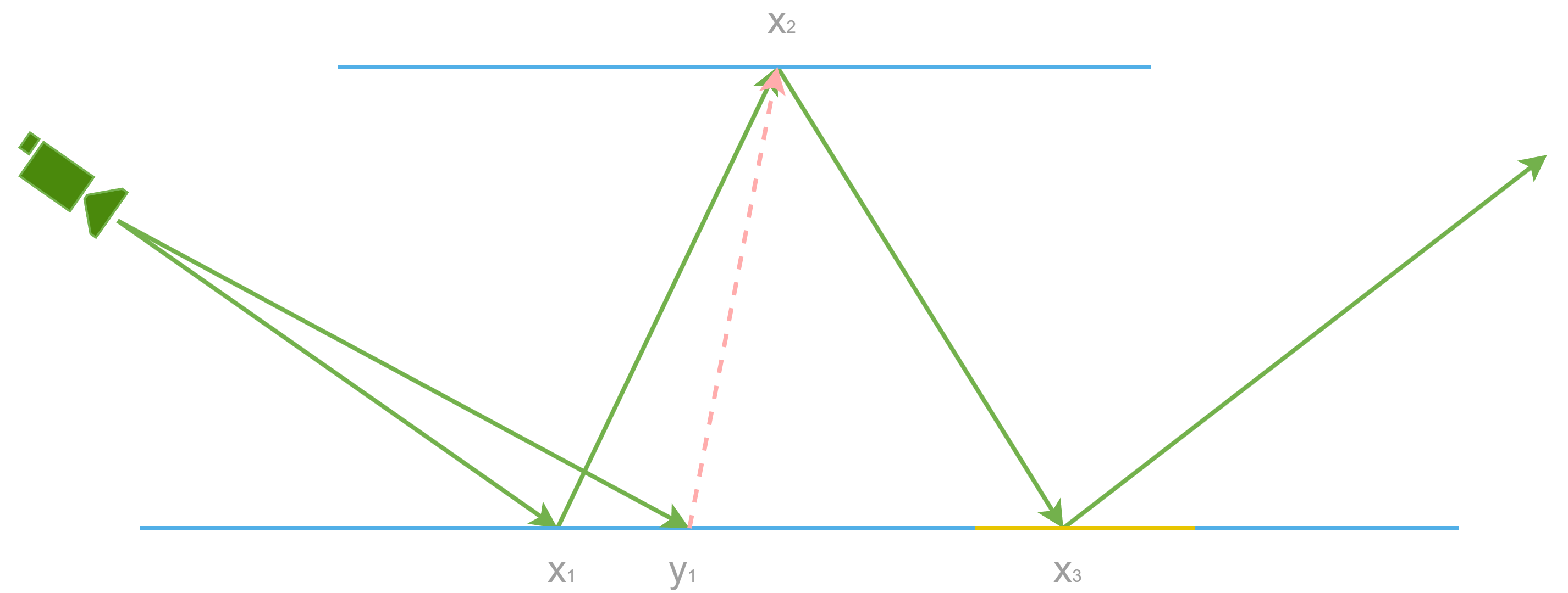
If our initial candidate is a path tree, the proposal PDF would be the PDF of producing the whole path tree. To reveal the problem, let’s expand equation 4 next, except this time, we will use a different representation of rendering equation for clarity.

This is essentially the same as equation 4, except that we are integrating over area rather than solid angle now. $V(x_1, x_2)$ is the binary visibility result between the two vertices. $\theta_{x_1 \rightarrow x_2}$ is the cosine value of the angle formed by the normal at $x_1$ and the direction from $x_1$ to $x_2$. The other $\theta$ should be pretty explanatory now. As we can easily notice, $L_l(x_2 \rightarrow x_1)$ itself is a recursive integral. Let’s expand it for a few times.

Let’s define the path depth as the number of bounces per path, where we count the light vertex(sample) as a bounce as well. For example, a path like this [$x_0 \rightarrow x_1 \rightarrow x_2 \rightarrow x_3$] has a depth of 3. Please be noted path depth definition may very likely be defined differently in other sources, which is fine as long as it is consistent in this post. Here $x_3$ should be either on emissive surface or a light source, including dirac delta light sources. Strictly speaking, in the context of discussion, $x_3$ won’t be dirac delta light sources, such as point or spot light, without NEE samples^[15] as continuation ray won’t hit them. Though, most path tracers draw NEE or BRDF samples for paths of each depth for faster convergence. To make things simpler, we assume our path tree don’t have those samples unless explicitly mentioned. With or without light samples, all of our theory in this post stands regardless. We will still call it a path tree without losing generality.

We can easily notice another $L$ in the equation 21, which means we can expand it similarly. And the process goes on without an end, which is why rendering equation involves an integral of infinite dimensions. Let’s define $L_k$ where $k$ is the only path depth we consider in the light evaluation. For example, if we only care about contributions from path of depth 3, we can simplify $L_3$ by combining equation 18, equation 20 and equation 21.

Correspondingly, we can figure out

For our convenience of later discussion, let’s isolate the integrand here.

With equation 23, we can rewrite equation 4 as below

If you are curious about why we can have inifite integrals in rendering equation with limited computing power, it is handled by Russian Roulette. We don’t really need to produce infinite number of paths if we stochastically choose to terminate after certain depth, which is what all path tracers do. It is also common for game engines to setup a max depth for paths so that there won’t be an infinite long tail thread tanking perf in corner cases. For simplicity of our discussion, let’s assume we have a max allowed depth $M$ and ignore Russian Roulette just to make our discussion a bit simpler. Of course, all of the theory below still holds when Russian Roulette is applied. With this simplification, our rendering equation for GI becomes

What equation 26 says is quite straight forward, the global illumination signal is essentially the combination of contribution from all paths whose depth are larger than 2. We purposely drop the arrow in $L_k$ here since it is not needed anymore, all we care about now is $L_k$ is a function of $x_0$ and $x_1$. A sample for Monte Carlo approximation of $L_k$ is as below.

ReSTIR GI only resamples everything from $x_2$, which is why we don’t count $x_0$ and $x_1$ in $\bar{\mathcal{X}}_k$. With the above context, we can define our initial candidate $\mathbb{T}$ in a more mathematical way now

Here is an important detail to point out. With our derivation here, there is actually a strong correlation between paths of different depth. Specifically, path of depth k is a sub path of path of depth k+1. Even though not drawing NEE or BRDF samples is rare, it is typical to see path tracers reuse the earlier path when producing longer path so that the time complexity of producing $M$ paths of different depth remains O($M$), rather than O($M^2$).

The PDF of producing a single path of depth $k$ is simply the product of all PDFs of producing each bounce. Here $p_a$ means the PDF w.r.t area.

In our context, the PDF of producing the whole path tree is simply the PDF of producing the longest path since we don’t have NEE or BRDF samples.

At this point, we have defined the exact form of our problem, which is equation 26. We also have a precise definition of our initial candidate in equation 28 and proposal PDF in equation 30. It seems that we could simply drop them in a regular Monte Carlo estimator ($\ell_k$ is defined in equation 24))

If we could have done so, the exact form of our proposal PDF is crystal clear and intuitive then. It would be $P(\mathbb{T})$. However, with a slightly deeper dive into the math, we can quickly notice a problem here.

Empirically, when we evaluate the unbiased light contribution of paths with a specific depth, we do not need to divide by the PDF of producing the whole path tree, we only care about the PDF of producing the paths with the specific depth. To see why equation 32 tells the truth more easily, let’s come up with a simpler example for now. Imagine we have the following integral of our interest.

We can easily come up with a Monte Carlo estimator like this

This is so simple that I’ll skip the proof that estimator 34 is both unbiased and consistent. But one thing that we so get used to is to divide by each sample’s own PDF in their own integral approximation. An analogue of the same mistake in equation 31 is to approximate $I_{simple}$ with the below estimator.

Here is a quick proof of why it is wrong.

Back to our own topic on equation 32, our problem here is not exactly the same as this simpler sample, but somewhat similar since they all divide extra PDFs. The idea is the same, we shouldn’t divide more PDF than we are supposed to. And we can easily derive the proof that the latter sum is the way to go, which means the former part clearly divides more PDF terms than necessary. To save some text, proof of this is left as a practice for readers.

If our initial candidates and proposal PDF won’t even work with naive form of Monte Carlo approximation, there is no theorical foundation for it to work in RIS or ReSTR anymore. We are hitting a deadend here with path tree being the initial candidate, we need to figure out an alternative solution next.

Primary Sample Space Initial Candidate?

The main problem in the above solution is that we divided extra PDF terms in each item of the sum in equation 31. To work around the problem, we must find a way to bake the corresponding path PDF in the approximation of each path contribution integral alone, rather than their sum. And we can try solving this by sampling in primary sample space. To see how it works, we need to redefine equation 23, except this time, we integrate over primary sample space.

Earlier we learned, the above revised form is exactly the same with the previous form that integrates over path domain in integral 23. Moving next, the input to the integrand in integral 39 will be the sample for one integral approximation in equation 26, which is simply a vector of ($u_2, \dots, u_k$),

We can think of the union of all such samples as the initial candidate. It is sort of a path tree, but in primary sample space. Precisely speaking, it is not a path tree anymore, it is merely a point in a high dimensional unit cube.

A nice feature of this setup is PDF of producing either $\mathbb{T}_{pss}$ or $\bar{\mathcal{U}}_k$ for any $k$ is exactly the same, they are simply 1. This is something that we didn’t have with the path space setup and the key to our problem as we can see later.

With our revisied version, the problem we are trying to solve becomes

Let’s see whether it works if we throw this initial candidate in a regular Monte Carlo estimator for approximation, we will then have this estimator

Quite different from last time, taking advantage of equation 42, we have the following derivation.

This says a lot! With our new setup, we can now call $\mathbb{T}_{pss}$ a sample. So we have successfully worked around the problem we saw in our last attempt. There is certainly some progress made here, we now can define our proposal candidates with proper proposal PDFs, which we are convinced that it works within a regular Monte Carlo estimation.

But what about in the context of RIS? Target function can simply be chosen the same as $\Sigma_{k=3}^M \ell_{pss,k}$. This target function makes a lot of sense as it is simply the integrand in the integral of our interest now, which in theory gives us zero-variance sampling with infinite initial candidate count. So yeah, it works as well.

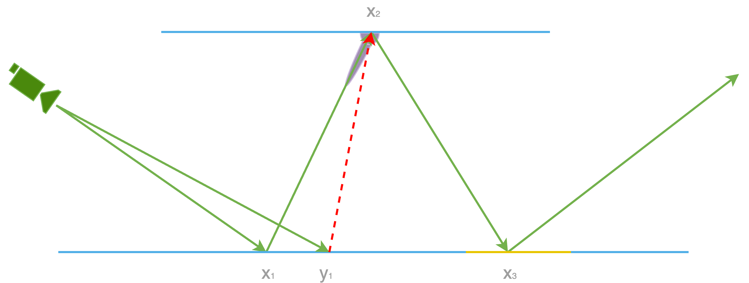
However, there is one subtlety that easily falls apart when we throw this theory in a ReSTIR GI implementation. ReSTIR gains its power by reusing samples. Here we defined a point in high dimensional unit cube as our sample, which is all what we can reuse, not much else.

What ReSTIR GI reconnects is $x_2$ in path domain, rather than primary sample space. With the above setup, the only thing closest to $x_2$ we have is $u_2$, the random number that we use to produce $x_2$. We certainly can’t simply reuse $u_2$ at $y_1$, which will produce a different $x_2$, none of the further bounces make sense if $x_2$ can’t be reused, unfortunately.

Our second attempt fails again as the theory is not sufficient enough to support what we actually want to do in ReSTIR GI even though it does work in a regular Monte Carlo estimator.

The Functional Form of Initial Candidates in ReSTIR GI

We explored the problems we faced with initial candidates in both path space (path with each bounce at surfaces of a scene) and primary sample space. Path tree as samples is clearly a failure as it won’t even work with a standard Monte Carlo approximation. Primary sample space solution allows us to make some progress to throw theory in regular Monte Carlo sampling, but not ReSTIR GI due to the lack of $x_2$ signal in the initial sample concept.

But we are making progress with primary sample space theory now. To fix the problem in the previous section, we can leave $x_2$ as is and the rest of the path tree in primary sample space. Hence, our integral now becomes this

Just as previous sections, let’s precisely define proposal candidate, proposal PDF and target function in ReSTIR GI so that we can evaluate the correctness of our solution. Initial proposal candidate in ReSTIR GI in this case is a point $x_2$ on surfaces of the scene and a point in a high dimensional unit cube. We can define sample as

Thanks to the path reuse between different depths, it still preserves the nice property that PDF of producing each path or the path tree is identical, except they are not 1 anymore.

Our new revised version of rendering equation now becomes

With all the nice properties preserved from both failed attempts made earlier, this looks good now. Our new estimator for equation 52 is

Same as above, let’s prove it working in a Monte Carlo estimation next.

As we can imagine, this gives us the theoretical support to throw such samples in RIS or ReSTIR. Our choice of target function could simply be $\Sigma_{k=3}^M \ell_{mix,k}$ this time since this is the integrand in our integral. This will in theory give us zero-variance approximation with unlimited number of initial proposal candidates.

Different from our second attempt, we can indeed share $x_2$ this time. Of course, this means we need to save some of the important bits of this bounce as well, such as normal and position. Besides, there is also some very minor catch with this new solution. In previous solution, we didn’t even need to store the proposal PDF at all. However, with this new solution, we need to introduce 4 more bytes in our reservoir data structure for $p_a(x_2)$, which is acceptable.

Unfortunately, there are still a few problems that we need to deal with with this idea before we can move forward.

Storing the sample {$x_2, u_3, \dots, u_M$} is expensive as the memory footprint of a reservoir is linear to the number of max depth supported in the path tracer. We need to not only store $M-2$ random numbers ($u_i$) in the path (again, it requires more if we draw NEE or BRDF samples), but also $M-2$ proposal PDFs that keep record of the PDF of producing each path. Proposal PDF here shouldn’t be a problem given that they are all simply $p_a(x_2)$. But just storing the random number $u_i$ per depth will still make reservoir’s memory cost O($M$). Large reservoir storage will not only require more bandwidth to read data from buffers, but also pressure on register usage as well, either of which is friendly to GPU performance. ReSTIR GI chooses to work around the problem by caching the radiance from $x_2$ to $x_1$. Strictly speaking, this is not possible as such a radiance is an integral itself, all we can do is to cache the unbiased approximation of the radiance from $x_2$ to $x_1$. To put it in math, here it is the cache form for path of depth $k$

Cached radiance estimate has a few major benefits. Since equation 55 is part of target function and rendering equation integrand in PSS as well, which are the only two places that requires the path sample as input, we no longer need to store the whole path anymore, we merely need the approximated radiance now. And during resampling or anywhere target function value or rendering equation value is needed, we can simply throw the cache over rather than reevaluating each of individual path contribution again.

This certainly gets us some progress by not requiring us to store the whole path anymore. But we still need to cache the approximated radiance from $x_2$ to $x_1$ for contributions of path of each depth, which we have up to $M-2$ possibilities in the worst case. The fact that our reservoir storage is O($M$) still remains. To work around this problem, we can take advantage of equation 54 again. Because the denominator is the same for all paths approximation, we only need to store the summed approximated radiance, rather for each depth. And this allows us to reduce the reservoir memory cost from O($M$) to O(1).

If we need to store all the random numbers in the reservoir for some reason, an alternative is to store the random number seed, which can reproduce the same sequence on every run. However, this approach imposes certain requirements on the implementation of the random number context. In contrast, caching the actual values enables faster evaluation of the target function or integrand during resampling, something that storing only the seed does not provide.

To be strict about the theory here, this cached solution is not flawless. If we take a closer look at the cached radiance estimate in equation 55, it is also a function of $x_1$. It means when we apply the cache on a path with a different $x_1$ during resampling, chances are our cached value is not 100% correct anymore unless the material at $x_2$ is simply lambert BRDF. There are two options we have here

• Reevaluate brdf at $x_2$. This has its own complication which we will mention later.
• Simply accept the bias, which is what most people do. And the original paper accepts this as well. Since ReSTIR GI is designed mostly for indirect diffuse and rough specular signal, this bias is totally acceptable in game rendering.

Typical Implementation of ReSTIR GI Initial Candidates

To be clear, the above mathematical model totally works. There is absolutely no problem that we can write a ReSTIR GI implementation based on the above theory. However, in reality, most people chose a different form of implementation, which is based on a slightly different mathemtical foundation than the above one. Specifically, the previous model uses all area PDFs to draw bounces in a path, rather than solid angle PDFs. We derived the theory this way as it involves slightly less complication.

Common sense is if we estimate an integral that integrates over area, rather than solid angle, we should use area PDF to draw the samples for real, which is not entirely true, but not totally nonsense either. I will point it out real use cases when it is not the case later. However, if we use the above model, the proposal PDF we store in a reservoir should be regarding to area rather than solid angle. Otherwise, it appears fairly confusing then.

Almost all implementations of a path tracer that I saw integrates over solid angle and store PDFs in solid angle form, rather than area^{[10, 16, 17]}. The typical way to find next bounce in a path is to shoot a continuation ray and find the closest intersection, rather than somehow find a point on the surfaces of the scene based on surface properties themselves.

To allow us storing solid angle proposal PDF in a reservoir, we need to make some minor tweaks to equation 47. Let’s define our final form of integral. Some of the math defined between equation 46 and equation 55, inclusive, in the previous section remain exactly the same. The things in the above derivation that need to be adjusted are equation 47, equation 48, equation 51 and equation 55. The revised definition are as below.

To clarify, from now on, when we mention these definitions, we use the new ones, rather than the old one defined in the last section. I could have listed all the definitions again, but that will only make the post longer. As we can see, most of the changes are pretty minor. To make sure we catch all the details here they are.

• In equation 56, we replace the G term with $cos(\theta_{x_1 \rightarrow x_2})$ as the other parts of G term help convert area PDF to solid angle PDF. Strictly speaking, we need to add visibility term in it. This complication is left for the next section when we talk about resampling.

• The multi-item product parts in equation 56 and equation 59 also have similar change. Superficially, they appear precisely the same with each other mathematically, it is not exactly true, which we will mention later in the post. Besides, there are two subtle details that are worth mentioning.

  • The visibility term in G term is ignored in the above equation. This is because we assume anything after $x_3$, including it, is found by a continuation ray, which means $y_{mix, i}$ and $y_{mix, i-1}$ are visible to each other for sure.

  • The PDF term $p_{\omega}(y_{mix, i-1} \rightarrow y_{mix, i})$ is the solid angle PDF around $y_{mix, i-1}$ to pick a direction to $y_{mix, i}$. A very important detail here is $x_{i-1}$ matters when we pick $x_i$. Later we will see this has quite some subtle implications on several things.

• The only change in equation 57 is we now integrate over solid angle for $x_2$ rather than area now, which means in a Monte Carlo path tracer, the PDF we divide needs to be w.r.t solid angle. And this is adjusted in equation 58.

With these subtle changes, it helps us understanding what exactly a ReSTIR GI implementation does now. Since most of the changes are so small, the above prove that this works in ReSTIR in its initial sampling pass still applies without any changes.

Before we move forward, here is a quick summary of what we came through so far.

• The integral is as equation 52, which is almost in primary sample space.
• The target function should be equation 56.
• The initial candidate in ReSTIR GI is the union of a point on surfaces of the scene and a point in a high dimensional unit cube.
• The PDF of producing initial candidate is simply the solid angle PDF of producing the bounce $x_2$.

The above items nicely answers the question we have at the beginning this section. At this point, readers should have a pretty solid understanding of what initial candidate in ReSTIR GI is, which allows us to talk about further details in resampling next.

Resampling Samples

Lots of the resampling theory in ReSTIR DI applies in ReSTIR GI as well, which will not be the focus of this section. In this section, we will only mention the delta between ReSTIR GI and ReSTIR DI, something I didn’t mention in my previous blog post.

Conversion of PDF during Resampling

In the original ReSTIR DI paper, area PDF was used to pick candidate samples on light sources. And area PDF is independent of primary intersection or the pixel that draws the candidate sample in the first place. While in ReSTIR GI, things are different. As we learn from the previous section, ReSTIR GI’s initial sample is $x_2$ and a point in a high dimensional unit cube. Even though the PDF of picking the high dimensional point is independent of $x_1$, we still need to figure out a way to pick $x_2$, which almost all ReSTIR GI implementation find by drawing a continuation ray based on BRDF at $x_1$. Typically, the PDF stored in GI reservoir is w.r.t solid angle around $x_1$ as well. And this means the PDF in reservoir is pixel dependent, unlike ReSTIR DI’s implementation. This adds a bit of complication when it comes to resampling as we can see later.

To be clear, the above statement only states how the original paper recommended implementing ReSTIR. This is by no means to say ReSTIR DI has to draw candidate samples based on area PDF, it doesn’t need to store PDF w.r.t area either. It is worth pointing out that it is not relevant between the stored PDF form and which form of PDF we use to draw our candidate samples. We could use solid angle PDF to draw candidate samples and store the corresponding area PDFs, vice versa. For example, on NvRTX branch of UE5, there are several methods besides area PDF sampling for drawing candidate samples on light sources, such as ReGIR^[18] and BRDF ray sampling. And we store ReSTIR DI proposal PDF w.r.t solid angle around $x_1$. And the same goes true for ReSTIR GI. Like I mentioned earlier, we could have totally came up with a solution that stored area PDF in GI reservoir in a ReSTIR GI implementation. Since most implementations store solid angle PDF, following discussion will assume so as well.

This subtle detail is critically important for us to implement ReSTIR GI correctly. Essentially, in equation 58, we pointed it out that $p_{\omega}(x_1 \rightarrow x_2)$ is actually a function of $x_1$. So what does it really mean to us when it comes to implementing ReSTIR GI.

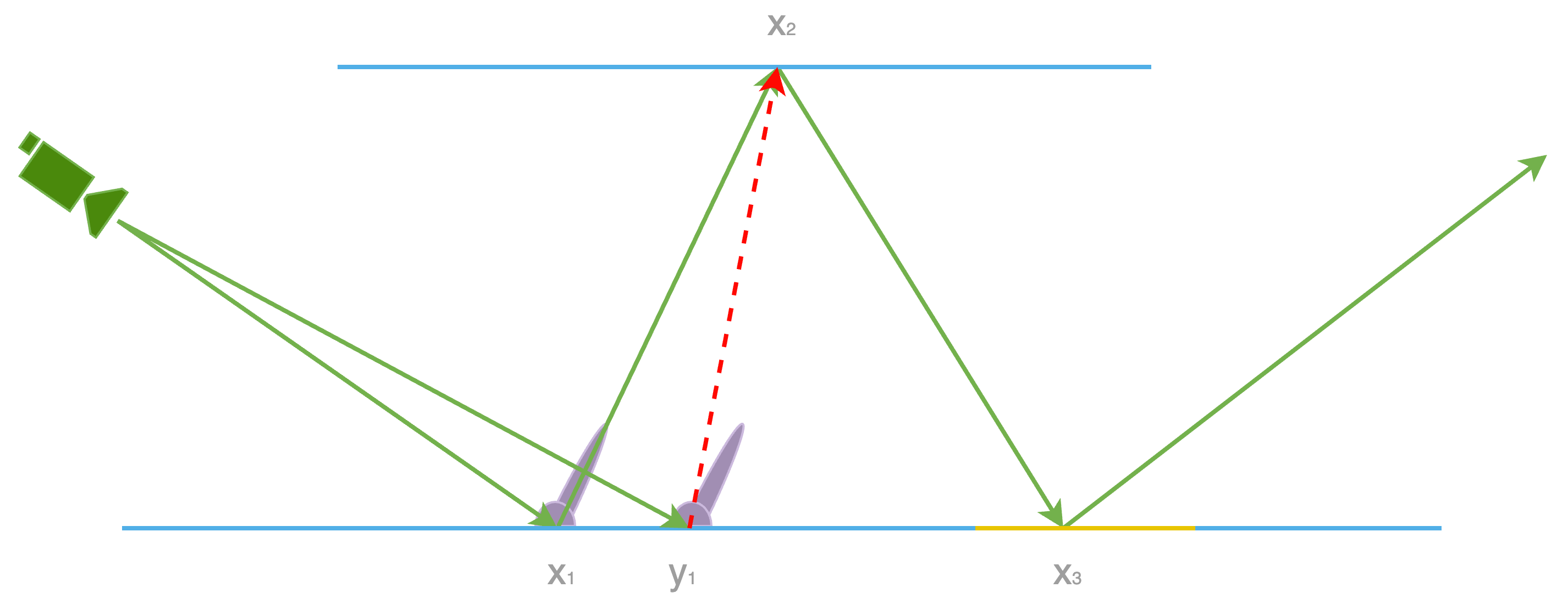
Let’s imagine a pixel B that hits $y_1$ would like to resample a candidate sample path drawn by a pixel A that hits $x_1$. During resampling, from pixel B’s perspective, this candidate sample $\bar{\mathcal{Y}_M}$ is drawn by some PDF. How this candidate sample is drawn doesn’t interest pixel B, all it cares is this sample comes with a PDF or a UCW. To make things simpler, let’s focus on PDF for now since we do know the PDF of picking this candidate sample even though in complicated cases, this PDF could be intractable, only UCW is known. The theory below applies to UCW as well.

We can certainly reuse the candidate sample. But can we directly reuse the PDF as well? It depends. If the PDF is independent of $x_1$, yes, we use the PDF without any changes. But if we draw samples based on a PDF w.r.t solid angle, it is a function of $x_1$. In order to resample this candidate path, we need a conversion to make sure we can transform $p_{\omega}(x_1 \rightarrow x_2)$ to $p_{\omega}(y_1 \rightarrow x_2)$. This appears intimidating in the first place. But it is actually quite trivial with the help of area PDF which is pixel independent. We can easily convert both into area PDF.

By combining equation 60 and equation 61, we can come up with the following equation.

To be clear, when we produce the resampling weight for this new candidate path, we need a few things, target function evaluated with this new candidate path mixed with $y_1$, multiple importance sampling weight and the reciprocal of proposal PDF and a Jacobian, the above transformation factor in equation 62. Here it is

This is well explained in the GRIS paper^[1]. But we didn’t use the GRIS theory for explaination here just to make sure readers who have no knowledge about it will still understand why such an extra term is needed.

One more note here is equation 63 draws a conflicted conclusion with Algorithm 4 in the original ReSTIR GI paper. After verifying with authors of the original paper, I believe the above form is the correct math for ReSTIR GI.

Biased Resampling

There could be multiple sources of bias in a ReSTIR GI implementation. In this section, I would like to chat about the cached approximated radiance. Let’s revisit equation 59 here. We mentioned the exact form of our cache, below is how we can reuse candidates from other reservoir:

The above shows how our cache will be in our Monte Carlo estimator. An observant reader may have already noticed a problem here, it is not even a correct expression to start with as $x_1$ is not part of the function, but it does show up on the right side. This moves the needle as when we resampling this candidate by another pixel, which has a different primary bounce, say $y_1$, the cache is immediately invalid as pointed out earlier unless it is purely lambert BRDF at $x_2$. To completely eliminate this bias, we need to reevaluate the BRDF at $x_2$ in equation 59 so that we can swap $x_1$ with $y_1$. At first glance, evaluating the BRDF at $x_2$ doesn’t seem difficult at all. The truth is quite the opposite. It is not trivial for a couple of reasons.

• Modern game engines have complicated material setup, which can be reflected by the size of GBuffer, a place holder for us to keep track of all relevant parameters for BRDFs. This is a very typical solution for rasterization^[19]. Lately, with the introduction of real time ray tracing^[20], a new form of container becomes the payload, which is a lot more memory sensitive than GBuffer. Typically, payload doesn’t have as much data as GBuffer because of it.
  If we would like to reevaluate BRDF at $x_2$ during resampling, we would need to store all necessary input for BRDF of our interests ideally. Even though, this is still O(1) memory cost, it does dramatically bump the size of a reservoir easily by a few times. Earlier we mentioned the extra memory bandwidth and register pressure, but an extra burden is possible heavier live state during Shader Execute Reordering (SER)^[21], none of which is friendly to GPU performance. The negative impact is no where near negligible.

• Apart from memory cost that burdens performance, there is also challenges coming from the BRDF execution logic. It could be quite a few of instructions just to evaluate a BRDF. Because this needs to happen at multiple places, wherever resampling weight is needed, shader divergence could be legit concern as well. Besides, the extra instructions in shader kernel may lower instruction cache hit rate as well. To be clear, we indeed have the BRDF evaluation cost during resampling because of target function require $f(x_2 \rightarrow x_1 \rightarrow x_0)$ if we choose our target function to be the full integrand of rendering equation. What I’m saying here is we don’t appreciate more execution of these unless we have to.

• With our current setup without any NEE or BRDF sampling, we got only one extra BRDF for evaluation, which is $f(x_3 \rightarrow x_2 \rightarrow x_1)$. The memory requirement goes beyond BRDF, it needs position of $x_3$ to be stored as well. But in practice, it is almost always more complicated than this. Because literally all path tracers draw NEE samples, which introduces another BRDF for evaluation. Things get even more sophisticated when multiple importance sampling with BRDF ray is applied, not just because we need one more BRDF evaluation for BRDF samples, but balance heuristic may easily introduce a few more. What is even worse is the NEE/BRDF sample positions will need to be stored as well.
  One practical and possible solution to the problem is to resample one single path within the path tree in path space and then pass the PSS candidate around, still with $x_2$ in path domain, of course. This is similar to what ReSTIR PT does. With care, if we resample one single path, it is possible to restrict the extra BRDF evaluation into one. This goes beyond the topic of this blog post, if readers are interested in it, checkout the ReSTIR PT paper^[1].

• If all the above still don’t convince you this is a bad idea, here is a blocker next. A candidate sample in ReSTIR GI is $\bar{\mathcal{Y}}_k$ during reusing, we only reuse $x_2$ in path domain. For the rest of the dimensions, we reuse the candidate sample in primary sample space. To some degree, we can think about it this way, we reuse $x_2$ and the random numbers ($u_3, \dots, u_M$) so that we can produce the rest of the path tree beyond $x_2$. The cache makes one assumption that as long as $x_2$ is reused, the same random numbers ($u_3, \dots, u_M$) will produce exactly the same path tree as the original path tree produced by the sample to be reused. But if we look closer, this assumption is a broken one. To explain, we draw BRDF continuation ray at $x_2$ to find $x_3$ during producing this candidate in the first place, this process again is a function of $x_1$. And this is pretty bad as with a different $y_1$ now, even if we have the same $x_2$, the rest of primary sample space candidate being the same doesn’t guarantee us the same path tree anymore. This means the bias not only comes from $f(x_3 \rightarrow x_2 \rightarrow x_1)$, but also a different path tree. The whole evaluation of this remapped candidate should be much more different than what we actually used to produce the cache.
  Do we have a solution to the problem? One way to fix the problem for real is to actually produce the newly remapped path tree by shooting a bunch of new rays with ($u_3, \dots, u_M$) and of course BRDF evaluations as well. This solution will work in theory. However, the power of ReSTIR is to borrow samples at minimal cost rather than drawing new samples. And this negates that by almost turning the resampling into drawing a whole new sample. This is not to say ReSTIR will lose its exponential growth of sample quality at linear cost, but it greatly reduces the number of candidates we consider during resampling. Be mindful if we check visibility during resampling in ReSTIR DI, reusing is similar with drawing a new sample in terms of cost. Different than ReSTIR DI, in ReSTIR GI, its initial candidate is a whole lot more expensive to produce, which commonly requires a path tracer. And this is why we can draw up to 32 samples in ReSTIR DI during initial sample generation pass, but we couldn’t produce anywhere near this in a ReSTIR GI algorithm.

With all the above reasons, it is clear that fixing the bias is close to impossible without tanking perf. But in theory, it is still doable. Even if we still want to give it a try, one more question we should be asking ourselves should be is there value in fixing it?

Imagine BRDF at $x_2$ has a sharp shape, what likely will happen is with reevaluated BRDF at $x_2$, chances are the new candidate will likely to be rejected, during resampling. This is simply caustic case, which is not something ReSTIR GI is designed for. ReSTIR GI will work mostly well when the BRDFs at $x_1$ and $x_2$ are mostly rough enough. In summary, when the BRDF at $x_2$ is sharp, the decision of whether to reevaluate during resampling it boils down to a choice between biased resampling and inefficient resampling, neither of which is perfect. In the case of rough BRDF at $x_2$, the reevaluated BRDF at $x_2$ likely will be similar with the one baked in the cache. This gives us another good reason not to pursue for a proper fix for this bias.

Visibility Check During Resampling

The next topic that we should visit is visibility checking during resampling. To make things clear, let’s add one more detail in equation 56

The revised form only differs by an additional visibility factor. This factor is commonly absent in most sources as it is mostly assumed that when rendering equation integral is over solid angle, rather than area, next bounces are found by continuation ray drawn from BRDF, hence consecutive bounces in a path are visible to each other by default.

However, I’d like to repeat my point here again, it is one thing that we integral over solid angle, it is totally another thing to draw samples from solid angle PDF. We don’t have to do so. There are a few examples already.

• As a matter of fact, ReSTIR GI itself is one example. During resampling, pixel B only borrows a sample from pixel A. What pixel A offers is a sample along with its PDF or UCW. But the way it produces its candidate sample could be based on PDF w.r.t solid angle around pixel A’s $x_1$, it could even be a sample produced by RIS, which only offers UCW, rather than PDF. Either is fine. However, the important detail to note is that for pixel B, the sample provided by pixel A is not drawn according to a PDF with respect to solid angle, at least not around pixel B’s primary bounce $y_1$, even if the rendering equation is integrated over solid angle. This could mean $y_1$ and $x_2$ may not be visible to each other, which makes the above visibility term necessary.
• If the above example is a bit difficult to understand, here is an easy one that everyone is familiar with. During NEE sampling, which commonly uses an area PDF, it doesn’t really matter if the rendering equation is over solid angle or not, a visibility ray, commonly named NEE ray or light ray, is necessary to make sure we don’t count contribution from blocked light sources. In this case, visibility ray is also needed.

One more subtle detail here is I didn’t add the visibility term between any other two consecutive bounces in a path in equation 65, this is by assuming continuation ray verifies it for us already, which is somewhat fine for ReSTIR GI. To be quite strict, ReSTIR GI doesn’t restrict in what way we should approximate radiance coming from $x_2$ to $x_1$ even though it mentions NEE sampling based path tracer, other methods can be used^[22]. For simplicity, we ignore it here by assuming further consecutive bounces after $x_2$ are all visible to each other by default. If necessary, this needs to be added.

So what does it mean with the extra visibility term in equation 65 when it comes to ReSTIR GI implementation? A few things

• We need to verify visibility during final evaluation. This sounds very nature because we would certainly not want to count blocked paths from contributing our pixel. The theory behind it is clearly explained in this section.
  And the truth is if the resampling path right before final evaluation checks visibility during its resampling, we don’t need to check it in the shading pass anymore as we are sure during the last resampling pass the winner sample is a visible path.
• Target function is a bit tricky here. Ideally, we need to count the visibility check during temporal and spatial resampling as well. This gives us zero variance approximation in an ideal world. However, this will lower the performance of resampling. So the question is can we choose not to check visibility just to save a bit of cost during resampling? Thanks to the per-initial candidate target function theory, we can choose to check visibility during resampling and we can also choose to ignore it during resampling in target function as well, which will lower sampling efficiency but gain some perf. We can even choose to do so based on particular samples to be reused.

In practice, not having to check visibility during resampling does allow us to reuse more samples during resampling, which is a welcome change in real time rendering. The efficiency lost mostly happens at where occlusion happens and denoiser commonly does a good job at getting rid of the noise in general.

ReSTIR GI Restrictions

Last, we should identify a restriction of ReSTIR GI. This is not a tech that solves all GI problems. As we can imagine, when BRDF at $y_1$ has a sharp shape, a tiny little change in the direction of the secondary bounce will likely result in no resampling at all. In a corner case, if it is a dirac delta BRDF at $x_1$, the path candidate for pixel A will only make sense for itself, any other pixels with attempts to reuse this sample will result in failure for resampling as the BRDF reevaluated at their own primary surface will result in 0 or a close-to-zero value, which commonly means zero or very small target function value, hence a lower resampling weight as well.

This is why ReSTIR GI is not specifically designed for sharp specular reflections in global illumination. Because in such cases, it effectively reduces to a standard path tracer. The quality of the sampling becomes identical to that produced by the path tracer during its initial sampling pass. As shown in the comparison below, we observe a significant improvement in GI quality on diffuse materials, while reflections in the mirror exhibit a similar level of noise.

Standard Path Tracer

ReSTIR GI

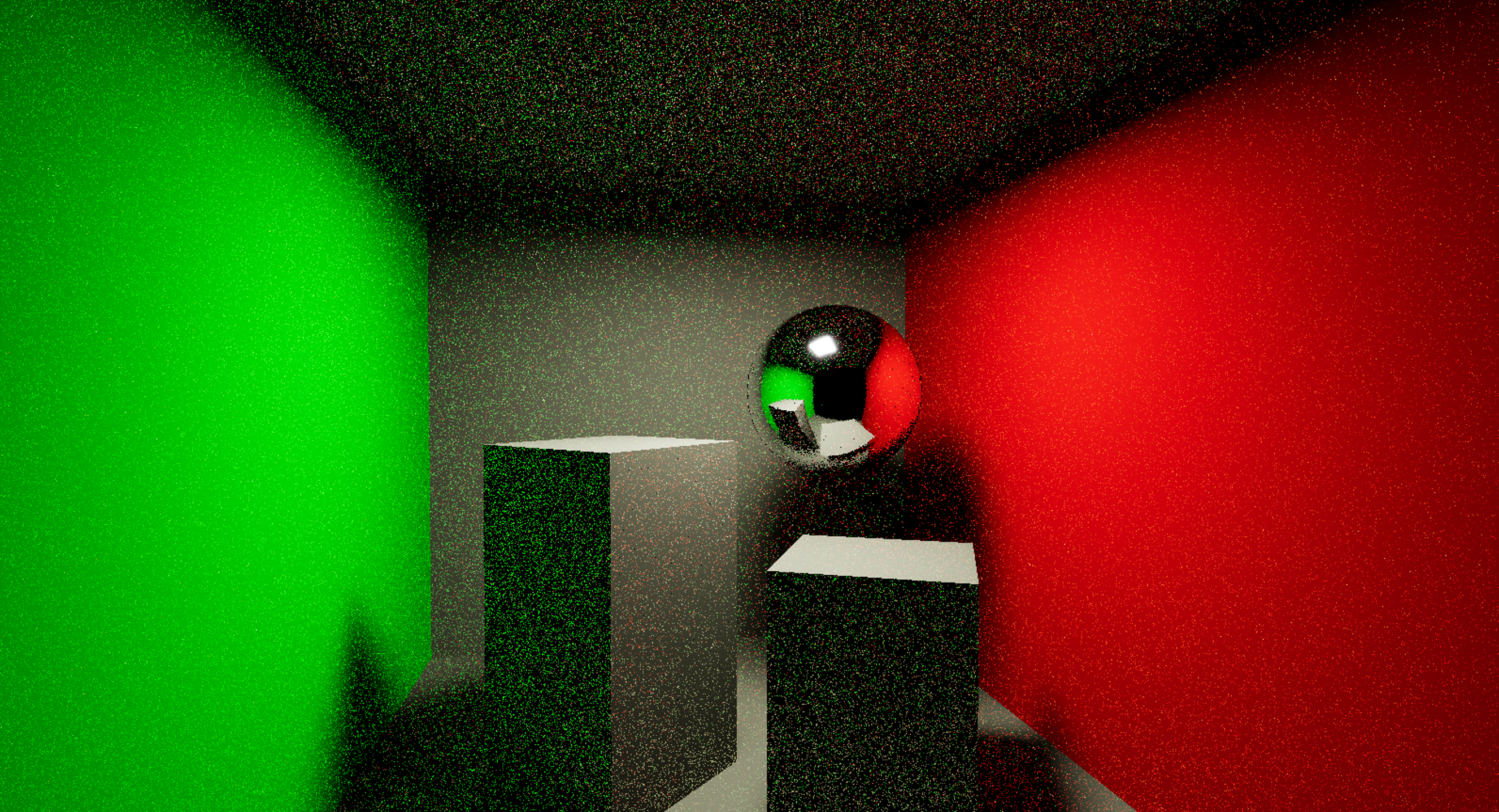
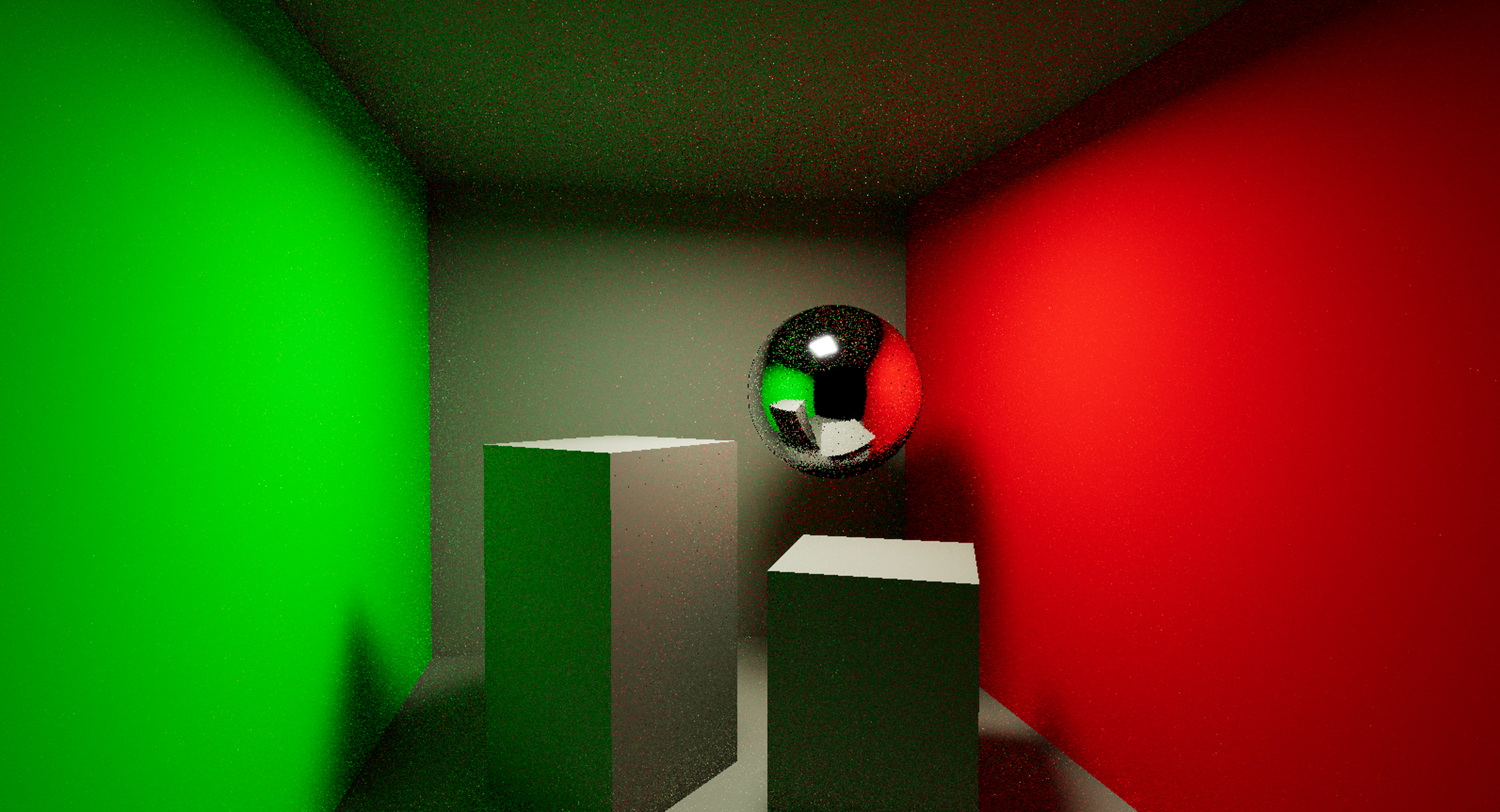
To clarify, this is not to suggest that ReSTIR GI cannot handle specular GI signals at all. In fact, based on my experience, any roughness value greater than 0.04 in UE5 will likely result in minimal issues during resampling. However, values close to 0.01 start to reveal sampling problems. In UE5’s Lumen system, the screen-space probe gathering pass also handles indirect diffuse and rough specular signals, making it an ideal candidate for ReSTIR GI to swap with. The following comparison of ReSTIR GI, with and without rough specular contribution, clearly demonstrates the value of the rough specular signal produced by ReSTIR GI.

Without Rough Specular Contribution

With Rough Specular Contribution

Summary

In this post, we’ve gone through an in-depth analysis of several key aspects of ReSTIR GI, including initial candidate concept, resampling, and the various sources of bias. These details are crucial when implementing the ReSTIR GI algorithm in a real project. While this knowledge might not directly improve your current implementation, gaining a deeper understanding of the underlying mathematics can open up new opportunities for future improvements.

Last but not least, before wrapping up this post, I’d like to thank my peer Markus Kettunen, one of the authors of the original ReSTIR GI paper, for helping me verify the theory and for reviewing this lengthy article with helpful corrections. He also pointed out the fourth cause in the bias section, which was new to me. That said, even though I received valuable input from my Nvidia colleague, this article is not an official explanation of ReSTIR GI. It simply reflects my personal thoughts and learnings during my implementation of ReSTIR GI. Please take everything discussed here with a grain of salt. And if you notice any inaccuracies or unclear explanations, feel free to leave a comment.

References