Ever since the introduction of RTX technology, the industry pushed really hard on real time GI solutions. ReStir (Reservoir Spatio-Temporal Importance Resampling) is one of the new popular topics lately. The algorithm can be applied in multiple applications, there are several different variations of the algorithm, like ReStir DI, ReStir GI, ReStir PT, Volumetric ReStir, etc.

The original papers are clearly the best resources to learn the tech. Due to the complexity of the algorithm, understanding the theory and math remains challenging for graphics programmers who are not very familiar with sampling methods. There are also a few blog posts ^{[5] [6]} available. However, there are still some fundamental mathematical questions not answered in the posts, which are fairly important for us to understand why the math works the way it does in ReStir.

In this blog post, rather than talking about the different variations of ReStir, I would like to talk about the very original method, ReStir DI. Different from existing blog posts, I would not mention any implementation details. The whole blog will be focusing on the mathematics behind the original ReStir, with more in-depth analysis of why it works. This should be a complementary reading of the original ReStir DI paper. It is highly recommended to go through the original paper first before start reading this post. Hopefully, after reading this post, readers would have a deeper understanding of how ReStir DI works mathematically.

Preliminary Reading

Since ReStir DI is not an easy algorithm to understand and lots of the details rely on some really basic theory. I think it makes a lot of sense to go through the basics first before starting to explain ReStir. So the first half of the post will be mainly about reviewing some fundamental concepts so that we would have a solid understanding of what is needed to understand ReStir.

Importance Sampling

This is the most fundamental concept in evaluating the rendering equation. Most of the details will be skipped as I would assume readers already have a decent understanding of it.

To evaluate the integral of $\int f(x) dx$, we would need to

• Draw N samples from a PDF
• Drop the N samples in the Monte Carlo estimator
  $I=\dfrac{1}{N} \Sigma_{i=1}^N f(x_i)/p(x_i)$

It is so easy to prove this that I would skip the math. If you would like to know how, check out my previous post here.

However, I would like to point out an important condition here. The support of p(x) has to cover the whole support of f(x). If it doesn’t, this can’t work.

To prove it, let’s say there is a sub-support in the f(x)’s support $\Omega$ that is not covered by p(x), naming it $\Omega_1$. This introduces a blind spot in the sampling’s support. Clearly, we have

Working out the math here

As we can see, we have a cut from the expected result. Intuitively explaining, this is because the estimator is no longer a function of any signal inside the support $\Omega_1$ anymore, while the target is a function of it. If anything is different inside that support, it would cause a different result integral while this change can’t be detected by the estimator as the PDF is unable to capture any signal there. Mathematically speaking, we can see that as long as $\int_{\Omega_1} f(x) dx$ is not zero, the result won’t be what we want. And it is almost not zero all the time. As a matter of fact, if we know beforehand, f(x) integrates to 0 over the support of $\Omega_1$, we would only need to evaluate the integral of the function in the support of $\Omega_0$ in the first place.

Multiple Importance Sampling

MIS is a common technique to improve sampling efficiency by taking multiple samples from different sources of PDFs, rather than just one. This method commonly improves sampling efficiency and can deal with integrals that are hard to approximate with one single source of PDF.

For MIS to be mathematically unbiased, it has to meet a few requirements. In the support of f(x),

• We must have $ \Sigma_{i=1}^M m_i(x) = 1 $
• $m_i(x)$ must be 0 whenever $p_i(x) = 0$

A hidden condition that is already implied by the above two conditions is that the union of the supports of all source PDFs must cover the support of f(x)

Since this post is about explaining ReStir, I would only put down some details that matters to ReStir. Other characteristics of MIS would be skipped. For a deeper explanation of MIS, please check out Eric Veach’s Thesis.

Mathematical Proof of MIS

In order to have a deeper understanding of this, let’s see how the math works under the hood first.

It is obvious that as long as it meets the first condition ($ \Sigma_{i=1}^M m_i(x) = 1 $), we would have an unbiased approximation of the integral of our interest.

For the implied requirement, since it is less relevant to ReStir, I would only put down some intuitive explanation here, leaving the math as a practice to readers (The proof should be fairly similar to what I showed in the previous section, but slightly more complicated). Same as the importance sampling blind spot issue mentioned above, if none of the PDF covers a sub-support of the integrand, it won’t pick up any changes in that support either, while changes in that support will indeed cause changes in the final result. This easily makes the estimate not accurate anymore.

However, this is by no means to say that all source PDF’s supports would have to cover the support of the function to be integrated. For any sub-support, as long as one of them covers it, it is good enough. Though there is one important condition, which is the second one mentioned above. Since it is slightly trickier to understand, I’ll put down the math proof here,

Let’s imagine for one PDF $p_k$, it has zero probability of taking a sample in a sub-support, $\Omega_1$. We can then divide the support of the function $\Omega$ into two parts $\Omega_0$ and $\Omega_1$. So we have

So let’s divide the previous MIS proof into two supports and see what happens,

What happens here is that our estimator has an extra cut from the expected value just like the importance sampling blind spot issue mentioned above. And this is exactly why we need to make sure we meet the second condition. If we do meet the second condition, what would happen is that the extra cut will be canceled because $m_k(x)$ is zero, leaving the rest parts precisely what we want. Making the estimator unbiased again.

As a side note, I would like to point out that in theory, we don’t really need to strictly meet the first or second condition to make the algorithm unbiased. There is a more generalized form

• First condition
  $\int \Sigma_{i=1}^M w(x) f(x) dx = \int f(x) dx$
• Second condition, assuming $\Omega_1$ is where $p_k$ is 0
  $\int_{\Omega_1} m_k(x) f(x) dx = 0$

However, in almost all contexts, it is a lot more tricky to meet this requirement without meeting the special form of them mentioned above. So this is rarely mentioned in most materials.

Commonly Used MIS Weight

Here I’d like to point out a few commonly used weight

• Balance Heuristic
  This is the most commonly used weight function in MIS. The mathematical form of the weight is quite simple, $ m_k(x) = N_k p_k(x) / \Sigma_{i=1}^{M} N_i p_i(x)$ . If we pay attention to the details, we would notice that it automatically fulfills the MIS conditions, which is very nice. Even though the weight looks quite simple, sometimes it can get quite complicated, like in the algorithm of Bidirectional Path Tracing. What is even worse is that sometimes the PDFs are not even tractable, making it impossible to use this method.
• Power Heuristic
  This weight is sort of similar to the balance heuristic, except it adds a power on top of each element in the nominator and denominator, leaving the math form like this $ m_k(x) = (N_k p_k(x))^\beta / \Sigma_{i=1}^{M} (N_i p_i(x))^{\beta}$. We can easily tell here that the balance heuristic is nothing but a special form of power heuristic when $\beta$ is simply one. And this weight also meets the MIS conditions as well. It is less commonly used compared with the balance heuristic, but it is indeed used in some cases for better sampling efficiency.
• Uniform Weight
  As its name implies, it is the same across all samples. Since it is constant and it has to meet the first condition, we can easily imagine what the weight is, it should simply be $ m_k(x) = {1}/{N_k} $.
  Not really meeting the second condition makes this weight seems to be pretty ridiculous at the beginning. As a matter of fact, if we use this weight, it possibly won’t reduce the fireflies at all, making this weight very unattractive. However, in the case where the PDFs are not even tractable, this is the only weight that we can consider using when it comes to MIS. And special attention is needed to make sure the method is unbiased. To counter the bias, we would need to count the number of PDFs that are non-zero at any specific sample and use that as the denominator, it would correct the bias then. Readers can try this idea in the math proof, it should be pretty easy to understand how it works.

Sample Importance Resampling (SIR)

Like inversion sampling, SIR is a method for drawing samples given a PDF. Though SIR requires way less from the target PDF itself. However, this method only approximates sampling the target pdf, it doesn’t really draw samples from the target PDF.

Given a target function $\hat{p}(x)$ to sample from, the basic workflow of SIR is as below

• Take M samples from a simpler and tractable PDF, we call this PDF proposal PDF, $p(x)$
• For each sample taken, we assign a weight for the sample, which is
  $ w(x) = {\hat{p}(x)}/{p(x)}$
• Next, draw a sample from this proposal sample set of M. The probability of each sample being picked is proportional to its weight. And throughout the rest of this post, this type of sample would be named as target sample.

The workflow is simple and straightforward. I’d like to point out a few different types of PDFs involved in this process

• Proposal PDF
  This is what we use to draw samples from in the first place. It should be tractable and cheap enough to take samples from as we would take multiple proposal samples from this PDF. I also want to point out that if this proposal PDF is expensive, it won’t have any impact on the unbiasedness of the algorithm though, except that it would need some extra treatment to avoid the cost. For example, in the work of ReStir GI, in order to generate a proposal sample, a ray needs to be shot, making it expensive, forcing the algorithm to take a lot less number of proposal samples compared with other variations of ReStir. The paper distributes the proposal samples across frames to achieve good performance.
• Target PDF
  We don’t really have the target pdf in SIR a lot of the times. What we have is target function. Target pdf is commonly recognized as normalized target function. Even though target function is what we used to assign the weight, it is not essentially different from using target pdf since a constant weight of the weights, the target function normalization factor, won’t have impact on SIR. Ideally, it shouldn’t be expensive either. Just like the proposal PDF, it could be.
  It is a nice property that we can use target function in place of target pdf, even if the target function is not normalized. Later we will see how this restriction doesn’t apply in target pdf.
• SIR PDF
  Some work called it real PDF. For consistency, I would call it SIR PDF throughout the whole post. This is the PDF that we are really drawing samples from. Clearly, we are not really drawing the final samples from the proposal PDF unless the number of proposal samples drawn is one. The truth is, unless the number of proposal samples is unlimited, we are not drawing from the target pdf either. We are actually drawing something in between, something that gradually converges to the target pdf from the proposal PDF as the number of proposal samples grows.

The graph below is a good demonstration of what will happen as M grows. The target pdf (green curve) is defined below. For better visual comparison, this target pdf is indeed a normalized distribution. Though it doesn’t have to be.

The proposal PDF (yellow curve) is simply

If you try dragging the slider from left to right, meaning more proposal samples are taken, it is obvious that the SIR PDF curve converges to the target pdf we would like to take samples from in the first place.

As we can see from the above graph, starting from uniform sampling, when the proposal sample count goes to 16, the SIR PDF is fairly close to what we want. Of course, this is simply a very trivial PDF, which we can even use inversion sampling to draw samples from. In other cases, things could be a lot more complicated. It could totally be possible a way larger set of proposal samples is needed for a good approximation of sampling the target pdf.

There are some pretty attractive characteristics of the sampling method

• Unlike inversion sampling, which is one of the most widely used methods, we do not need any knowledge about the target pdf, apart from that we must be able to evaluate it given a sample. This alone gives us a lot of flexibility in choosing the target PDF.
• What makes the algorithm even more attractive is that we can even add a constant scaling factor on the target PDF as the algorithm would be the same. A relative scaling factor on all weights would mean no scaling factor applied at all. To explain it a bit, imagine we have two proposal samples with their corresponding weights being 2.0 and 8.0. The chance of picking the first sample are 20%. If we scale the target pdf by 5.0, the weights will be 10.0 and 40.0, resulting in exactly the same chances of picking each sample as well.
  This offers an extra level of freedom for us to choose our target PDF as a lot of the time we can’t really normalize our target PDF. This opens the door for us to choose literally any function we would like to use, rather than a PDF that has to integrate to 1 in its support.

With all these limitations gone, it is not hard to imagine the value of SIR. It offers us a powerful tool to draw samples from distributions that we couldn’t sample with other methods, for example, the rendering equation itself. If we can take samples from a PDF that is proportional to $L(w_i) f_r(w_i, w_o) cos(\theta_i)$, we really just need one single sample to solve the rendering equation without any noise. This is really hard for traditional methods, like inversion sampling and rejection sampling. Because the distribution is not even a PDF, there is no easy way to normalize the distribution. Normalizing the distribution requires us to evaluate the integral in the first place, this is a chicken and egg problem itself. However, just because we can’t draw samples from this distribution doesn’t prevent us from approximating drawing a sample from it using SIR. This is exactly what ReStir GI does.

With these limitations gone, it seems that we have the power to sample from any distribution now. However, there are clearly some downsides of this algorithm as well

• The biggest downside of this SIR method is that it is unfortunately intractable. To be more specific, it means that we don’t really have a closed form of the SIR pdf that we take samples from given a specific M, proposal PDF, and target function.
• There is a big issue because of the intractable nature of the SIR PDF. Given a random sample taken from somewhere else, we can’t easily know the probability of taking this given sample with this SIR method.
  To illustrate why it matters, if we take a re-visit of the previous MIS balance heuristic weight mentioned above. We can quickly realize that balance heuristic is not possible as long as one single PDF is a SIR pdf, meaning we take one single sample with this SIR method as the samples in MIS, balance heuristic is not an option anymore.
• Sometimes it would require a big number of proposal samples to achieve a good approximation of sampling the target pdf. This could be a deal breaker as generating a huge number of proposal samples doesn’t sound cheap itself. ReStir solves this problem by reusing sample signals from temporal history and neighbors, which greatly reduces the number of real proposal samples needed to be taken per-pixel.

Resampled Importance Sampling (RIS)

RIS is a technique that takes advantage of SIR to approximate the integral in an unbiased manner. It comes with a complete solution to approximate the integral without any bias, while SIR only cares about drawing a sample.

To evaluate $\int f(x)dx$, RIS works as followings

• Find a proposal pdf p(x) that is easy to draw samples from and draw M samples using this PDF.
• Find a target function $\hat{p}(x)$ that suits the function well
• For each proposal sample, assign a weight for it, $w(x)=\hat{p}(x)/(p(x) M)$
• Draw N samples (y) from the proposal sample set (x) with replacement, the probability of each proposal sample being taken should be proportional to its weight. Replacement means that the N samples taken out of the proposal sample set could be duplicated. This simplifies the problem into taking one sample based on the weights and repeating the process N times.
• Then we use the N samples to evaluate the integral approximation, but with a bias correction factor, which is $\Sigma_{i=1}^{M} w_i(x_i)$

Please be noted that the weight here is slightly different from the previously mentioned weight. This is fine as scaling the target function is allowed in both SIR and RIS. But the below function has to skip the 1/M part since it is merged into the weights already.

The final form of our Monte Carlo estimator would be as below

Here $y_i$ is only a subset of $x_{ij}$. The way $y_i$ is picked can either be done through a binary search or linear processing like Reservoir algorithm. Binary search would require us to pre-process the proposal samples beforehand, which is not practical in the context of ReStir though.

There are some requirements for this method as well

• M and N have to be both larger than 0.
  It is quite easy to understand this. If either the proposal sample count or the target sample count is zero, we are not really doing anything here.
• In the support of f(x), both $\hat{p}(x)$ and p(x) have to be larger than zero as well.
  This is not hard to understand as well. If either of the PDFs is zero in a sub-support, what happens is that the SIR method would have no chance to pick samples from that support at all. And this is precisely the blind spot issue mentioned above in the Importance Sampling section.

To Make it a bit easier to understand the workflow below is a graph demonstrating how it works

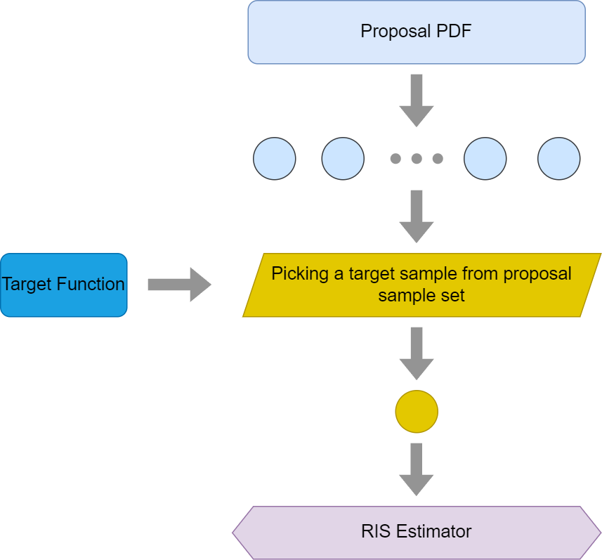
Please notice that the SIR algorithm only generates one target sample and feeds it into the RIS estimator. The theory explained in this blog post would also work for cases where multiple target samples are sampled. However, since the original paper only uses one target sample in its explanation, I’d like to stick to its implementation for making things simpler to understand.

MIS used with RIS

Whenever it comes to multiple importance sampling, there are two ways that it could be used with RIS.

The first option is when taking proposal samples from the proposal PDFs, there is really nothing that prevents us from drawing samples from different PDFs. In the previous section, we mentioned that all the proposal samples are coming from a same proposal PDF. There is no such limitation. We could draw samples from multiple different PDFs if we want to. Though, it is critically important to make sure the conditions of the MIS are met properly.

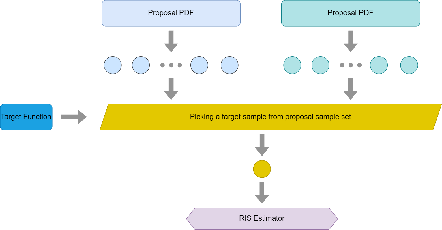
As pointed out in the GRIS paper, the weight for each proposal pdf could be generalized to this form

It is not hard to realize that the previous weight is nothing but a special form of this generalized form where the MIS weight is simply uniform weight and the proposal PDF is all the same. Since that weight is a MIS weight, it has to make sure it would meet the two conditions involving weight in the MIS algorithm. Otherwise, it could introduce bias.

Below is a graph demonstrating the workflow for MIS used in RIS.

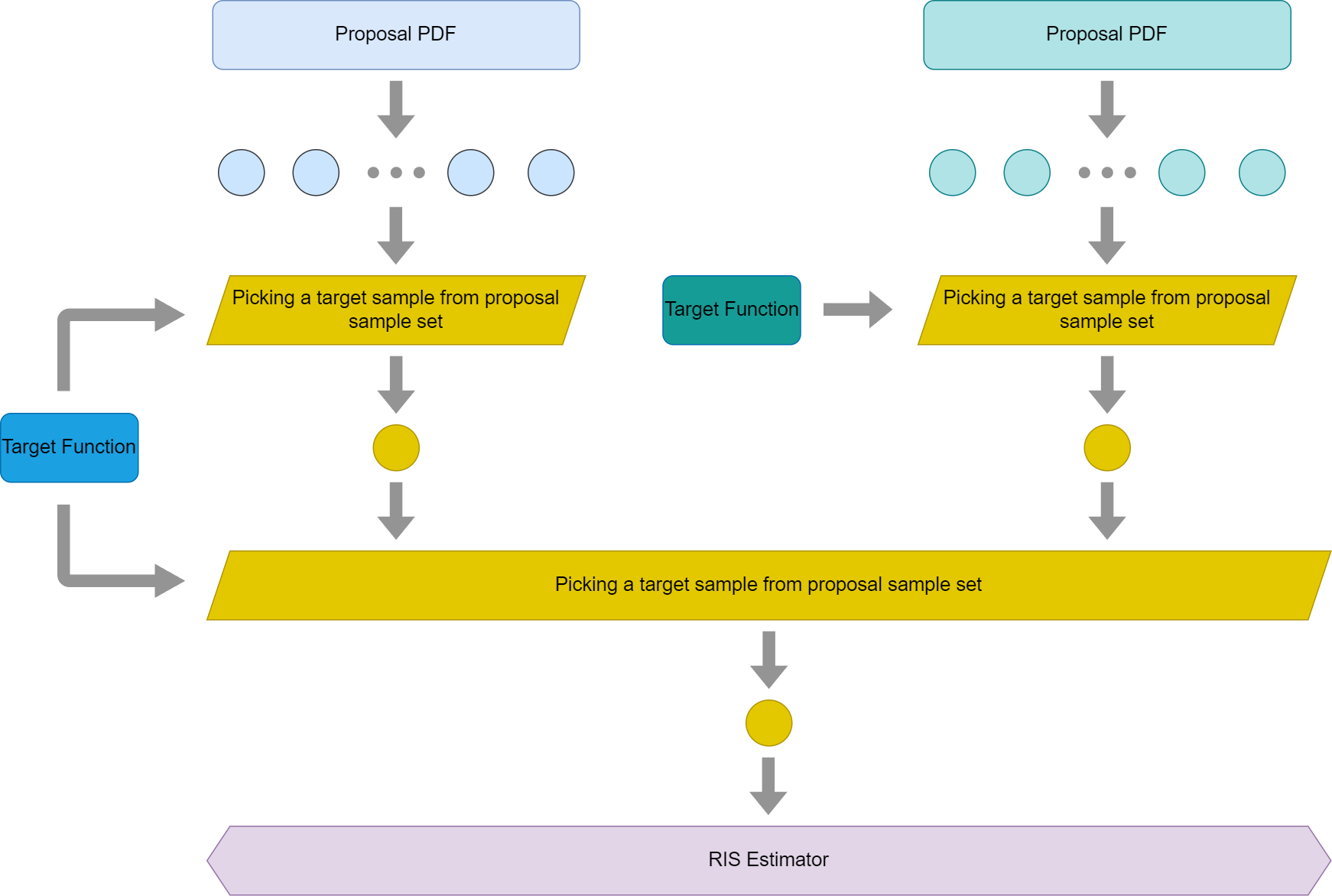
Another usage of MIS with RIS is to treat SIR as an individual sampling method itself. So target samples drawn from different SIR methods could be used as different samples drawn from different PDFs in MIS. Put in another way, we essentially treat different SIRs as different PDFs in MIS. From the perspective of MIS estimator, it doesn’t really care about whether the sample is drawn from one SIR or another, or maybe even from a different method, like inversion sampling. However, there is one tricky thing to point out, as balance heuristics would require evaluating samples on all PDFs, since SIR’s PDF is not even tractable, it would be difficult to use balance heuristics as weight.

Same as before, here is a diagram showing how we can treat RIS as a regular sampling method in MIS.

Math Proof of RIS

For those readers who don’t like taking things for granted, to fully understand the RIS method, it is necessary to understand why it is unbiased. There is very clear proof of it mentioned in the appendix of Talbot’s paper.

Rather than repeating his derivation, I would like to put down another slightly different proof, which is similar to what the ReStir DI paper does when it talks about the biasness of the ReStir method.

Since the original samples come from the proposal PDF(s), target samples are merely a subset of proposal samples without introducing new signals to the evaluation, we would only need to integrate the support of the proposal samples to get the approximation.

To simplify our derivation, let’s define a few terms first

Please notice that without losing generosity, I used different proposal PDFs here. To prove the RIS with same proposal PDF, we simply need to get rid of the subscript of $w_i(x)$.

As we can see from the above derivation, lots of the items cancel, leaving a very simple form, the exact result that we would like to approximate in the first place. With this proof, we can easily see that it doesn’t matter if RIS picks proposal samples from different PDFs, this is exactly how MIS works in RIS in the first method I mentioned above.

Nice Properties of RIS

Before moving to the next section, let’s summarize some of the nice properties of RIS.

• There isn’t that much needed between the proposal PDF and target function, offering a lot of flexibility in terms of choosing the best PDF/distribution for your application. The only thing that is required is that they have to both cover the support of target function f(x). To be more specific, if we are sampling from different proposal PDFs, the union of the supports of all proposal PDFs would need to cover the whole target function’s support. If one of the proposal PDFs doesn’t cover the full target function’s support, it is fine as long as the MIS weight is properly adjusted. Of course, the target function’s support should be a superset of the integrand’s support as well.
• This was mentioned in the previous section. I would like to emphasize it again since it is something important. The target function used in RIS doesn’t need to be a normalized PDF at all. It can literally be anything. As a matter of fact, ReStir DI algorithm uses the unshadowed light contribution, $L(w_i)f_r(w_o,w_i)cos(\theta_i)$, as target function. With traditional sampling methods, it is very hard as this distribution is hardly a PDF itself.
  To see how it works in math, in the previous derivation, we can easily notice that the value of $W/\hat{p}(x)$ does not change when we scale target function since it is both in the denominator and nominator.
• As we mentioned before, the supports of the target function and proposal PDF both cover the support of f(x). We can take advantage of this fact to predict if the SIR PDF is zero by inspecting target function and proposal PDF even if SIR PDF is intractable. This is a useful feature that we would take advantage to counter the bias in ReStir DI.

Weighted Reservoir Sampling (WRS)

The second step of SIR algorithm requires us to pick a sample from all proposal samples and each sample’s probability of being picked is proportional to its weight. This application easily reminds us of a binary search algorithm with a prefix sum table. However, even if the time complexity is only O(lg(N)), the preprocessing step’s time complexity is still O(N). It would be suitable for cases where data is more static and can be preprocessed and used multiple times later, like HDRI sky importance sampling. In a more dynamic environment, it is less practical as the bottleneck will be O(N) during preprocessing. And it also requires O(N) space as well, which is another deal breaker for efficient SIR sampling. All these issues require us to seek an alternative solution, which is where WRS chimes in.

Weighted reservoir sampling is an elegant algorithm that draws a sample from a stream of samples without pre-existed knowledge about how many samples are coming. Each sample in the stream would stand a chance that is proportional to its weight to be picked as the winner. For example, if we have three samples A, B, C, with their corresponding weight as 1.0, 2.0, 5.0, there will be 12.5% chance that A will be picked, 25% chance that B will be picked and 62.5% chance that C will be picked. Besides, if there is a fourth sample D coming even if after the WRS is executed, the algorithm is flexible enough to take the fourth sample in without breaking the rule that each sample would have a chance proportional to its weight of being picked. And what makes it even more attractive is that it only requires O(1) space, rather than linear space. There are certainly more attractive properties of this algorithm, which we would mention at the end of this section after learning how the math works first.

To be clear, there are certainly variations of WRS existed. For example, the algorithm could actually pick multiple samples rather than just one of them among the set. However, this is the only version we care about in ReStir DI as ReStir DI requires sampling proposal sample set with replacement. So all we need to do is to repeat the above algorithm multiple times. Though, there may be a more optimized algorithm existing to pick samples with replacement. But this is out of the scope of the topic in this post.

In order to implement the algorithm, we would need to define a reservoir structure with a few necessary fields

• Current picked sample
• Total processed weight

An empty reservoir would have none as the current picked sample and 0 as total processed weight.

Please be noted that these are the only two fields required for WRS algorithm. ReStir DI does require another field, which is the number of samples processed so far. But since this section is all about WRS, the processed sample count is ignored to avoid confusion.

The basic workflow of WRS goes like this. For an incoming sample, it would either take the sample or ignore the sample depending on a random choice. A random number between 0 and 1 is drawn. If it is larger than a threshold, which is defined this way

The incoming sample will be ignored. Otherwise, the new sample will be picked as the winner replacing the previously picked sample, if existed. Regardless, the total weight will be updated accordingly. A side note here, pay special attention when your random number equals the threshold. This could be problematic depending on how we would like to deal with the incoming sample when it is equal.

• If we would like to pick it when it is equal, there is a non-zero chance to pick incoming samples with zero weight.
• If we would like to ignore it when it is equal, there is a non-zero chance that we would ignore the first sample, which should have always been picked.
• If the first sample has zero weight, which is totally possible, accepting this sample or not is a choice of personal preference then.

How to deal with this sort of corner case is left to the readers as an exercise as this is not exactly what this post is about. But be sure to deal with this situation when implementing the algorithm to avoid weight bugs.

Mathematics Proof

Compare with the previous math proof, this one is a lot simpler and requires nothing but junior high math.

To prove how it works, let’s start with the first incoming sample with non-zero weight in the WRS algorithm. We don’t care about the first few samples with zero weight, we can pretend they don’t exist. What will happen for sure is that the incoming sample will be taken as the random number will not be larger than the threshold, which is 1.0, forcing the new sample to be picked. And this indeed matches our expectation as if we only have one sample, the probability of this sample being picked is 100%.

So assuming the algorithm works after processing N incoming samples, this is to assume that after processing N samples, each visited sample stands a chance of being picked that is precisely this

As the way WRS works, we do have the denominator nicely recorded in a single variable

Let’s see what would happen when a new sample comes in. If the random number is smaller than the threshold mentioned above, the newcomer will be picked. This means that the probability of the new sample being picked is

And this probability is exactly what we want for the new sample to be picked. And there is also a chance that the new sample will not be picked, which is

So each of the previous samples being picked is reduced by the risk of the new sample could be picked. And the probability goes down by exactly the above factor, leaving each of the previous samples standing a chance of this being picked,

And this probability again is also what we want for each of the old samples to hold to be picked.

At this point, we can easily see that if WRS works for N incoming samples, it would work for N + 1 samples as well. Since we also proved that it indeed works when N is 1, it would mean by thinking it recursively, it would work for any number of incoming samples.

Treating a New Sample as a Reservoir

As we previously mentioned, the reservoir structure really only needs to hold two members, the total processed weight and the picked sample. And if we think about each new sample, it really just has a weight. However, we can also regard a new sample as a mini reservoir with the sample itself picked and the total weight equals the sample weight. From this perspective, there is no individual sample any more, everything is a reservoir. And the WRS algorithm would simply use the tracked reservoir and takes a new single sample reservoir.

So the question is, can WRS also take reservoirs generated by other WRS execution, rather than just a single sample reservoir?

Fortunately, the answer is yes. Let’s say the WRS has processed N samples so far and it takes an incoming reservoir as its next input. If the incoming reservoir has processed M samples first, each sample in the visited M samples would stand a chance of this of being picked

I purposely used y here to indicate it is a different source of samples. Dropping it in the current reservoir processing, we would have each of the previously visited samples having this chance to be picked

So after being processed by the WRS algorithm, each of the previously visited M samples would have the correct probability to be picked as a whole. Even though this is done in two passes, rather than the previously mentioned one-pass algorithm.

W.r.t the visited N samples, their probability of being picked is also reduced by this factor

Applying this to the existing probability, we will have each visited sample having this chance of being picked

This nicely matches our expectations as well. So at this point, we can safely draw the conclusion that WRS can be performed in multiple recursive passes, it won’t have any impact on the probability of each sample being picked. It is also not hard to see that this recursive process certainly doesn’t get limited by two levels.

Nice Properties of WRS

Now we know the math behind this algorithm as well, it is time to summarize what properties we can take advantage later

• WRS doesn’t need to know the number of samples during its execution. It takes a stream of inputs, rather than a fixed array of inputs.
• WRS has O(1) space requirement even if the processed samples could be millions. It also requires only O(1) time to process each input, even if the input is a reservoir with millions of samples processed.
• WRS supports divide and concur. Imagine there is a source of a million samples, we can first divide them into multiple trunks and process each trunk on a different CPU thread. The order of each trunk being processed is irrelevant. After every thread is finished, we can resolve the result with a final gather pass. How and when we divide won’t have any impact on the probabilities at all.

ReStir DI Introduction

With all the above context explained, we are now in a good position to move forward to discuss the detailed choices made by ReStir DI.

Before doing it, I would like to give a brief introduction of what ReStir DI is and what problem it tries to tackle. It is highly recommended to read the original ReStir paper to get all the details.

Targeted Problem

The original ReStir DI algorithm focuses on tackling the many light problem. More specifically, whenever an intersection is found and shading operation is needed, we would first need to pick a light among all light candidates to take samples from. There are several obvious options for toy renderers,

• The most straightforward algorithm to pick a light is to randomly pick one light with equal probability for each light. Even though it doesn’t sound very promising, it can be done in O(1) time and requires almost no pre-processing.
• We could also construct weights by taking some factors into account when picking lights, like the emissive power of the light. As long as those factors are not shading point dependent, we could pre-calculate a table first and use binary search to find a light proporition to the weight. Pbrt 2nd uses this method for sampling a light.
• If the weights are shading point dependent, it commonly means that we would need to iterate through all lights to get a good sample. However, this is clearly a deal breaker for setups with millions of lights, it wouldn’t even work for hundreds of lights practically since iterating through all lights is a per-pixel operation.

Of course, the above methods are the most trivial and fundamental solutions available. There is some existing work exploring different ideas in this domain ^{[12] [13] [14]} , etc. Among all of the existing work, ReStir DI scales really well, up to millions of lights. And it is also quite practical to implement on modern graphics hardware, especially Nvidia RTX cards. Strictly speaking, ReStir DI not only finds a good light candidate for shading, but also finds a good light sample. There is still subtle differences between sampling a light and sampling a light sample.

• The former only cares about picking a light out of many, which would still require us to pick a sample on this light later. And in some situations, it could be quite tricky. For example, when the light is a huge area light and the brdf is very spicky there could be risk in producing lots of fireflies.
• On the other hand, sampling a light sample offers enough signal for the rest of the algorithm to simply take over. Since ReStir does pick quality sample in an efficient manner, the aforementioned problem simply doesn’t exist in it.

Basic Algorithm Workflow

The algorithm works for rendering 2D images. It works so efficiently that it could render in real time. Each pixel would keep track of its own reservoir across frames.

Below is a very brief introduction of the workflow

• For every pixel on the screen, it first takes multiple initial light samples (M = 32 in their implementations). These light samples are treated as the proposal samples, which would later be used in RIS algorithm.
  In order to take the proposal samples, ReStir DI first pick a light randomly with the probability of each light being picked proportional to its emissive power. If there is HDRI sky, a 25% probability is given to it by default. As mentioned before, since the probability is proportional to its weight not the shading point, the algorithm could use the traditional binary search method for picking a light. And once the light is picked, a corresponding method is used for generating a random light sample on the light source based on whether it is a HDRI light or an area light.
  All of the proposal samples will be processed in RIS algorithm through weighted reservoir sampling. The target function is unshadowed light contribution. Mathematically, it is $L(w_i,w_o) f_r(w_o,w_i) cos(\theta_i)$, except that we don’t know if the light is visible to the shaded point or not.

• An optional visibility reuse phase could be done here. This is introduced because even with unlimited number of proposal samples, the result could still be noisy due to the gap between the target function and the rendering equation, specificially, the visibility function. By introducing a visibility check here, we could use the real rendering equation (the integral part) as our target function, resulting in much less noise caused by visibility issues. If this algorithm is used, the algorithm would need to check visibility during neighbor target sample merging as well to preserve its unbiasness.
  This is an optional phase as it could introduce big performance impact due to a larger set of rays shot each pixel.

• The second phase in the algorithm is temporal reuse. With some motion vector, the algorithm could find itself in the history of rendering the previous frames. And it combines the reservoir that belongs to the corresponding pixel in the previous frame. Just like TAA algorithm that improves the image quality by distributing cost of super sampling across multiple frames, the temporal reuse does exactly the same thing.

• In the third phase, the algorithm could repeat in multiple iterations. In each iteration, it would try to find a random neighbor and combine its reservoir as well.
  This is where the number of indirectly visited proposal samples for each pixel will soar. Imagine there is n iterations, k neighbors are picked. To make things simpler, let’s consider only the first frame. Each pixel after this phase would see $(k + 1) * M$ visited proposal samples. With multiple iterations, the theoretical maximum number of visited samples could be as high as $(k + 1)^n * M$. However, this is only at the cost of O(nk + M).

  • Since there is quite a good chance that visited proposal samples would be revisited indirectly again, it would be hard to reach to the theoretical maximum for this number. And this is why after several iterations, we get diminishing return in terms of quality.
  • Please notice that I mentioned ‘indirectly visited proposal sample’. One important detail I’d like to point out is that this is by no means to say your current pixel’s RIS would visit this number of proposal samples, it actually ‘visited’ them in a recursive manner indirectly. Quality-wise, it could be something similar, but not exactly the same thing. We’ll explain this later.

  This is just about the first frame as the temporal reuse doesn’t bring anything useful due to the lack of history. But for later frames, temporal reuse will introduce way more signal only at O(1) time. With temporal reuse, it gains a second chance to make the number grow even faster.

• With all the three phases, the pixel now has a winner light sample, which survived among potentially millions of samples, easily making it a high-quality light sample. And the algorithm then uses RIS method to evaluate the light contribution here. It is only in here that a shadow ray is traced so the cost of the algorithm is totally within the capability of the modern hardware.

This same process is repeated every frame. As frame goes, each pixel essentially visits millions of proposal samples in their RIS algorithm eventually resulting in drawing samples quite close to the target pdf, the unshadowed light contribution.

The above explanation really serves as a review of the algorithm to readers who read the paper. It could be a bit confusing for people who don’t know the algorithm.

Common Confusion in Understanding ReStir

After my first time reading through the paper, I had a lot of confusion.

• The math in the paper assumes the proposal PDFs are all the same. Even if the PDF for taking light candidate is exactly the same for all pixels’ RIS execution, the PDF of taking initial light samples is the product of the PDF of picking a light candidate and the PDF of taking a light sample from the light candidate, the latter of which is not the same for all pixels. So does the implementation really uses one single PDF to take light samples?
• I had a really hard time to be convinced this is unbiased, especially the sampling neighbor part since the neighbor pixel’s RIS algorithm essentially uses a different target function than the current pixel.
• The paper has a very clear explanation and proof that the expectation of the big W (the sum of all weights divided by target function and the number of visited proposal samples) is the reciprocal of the SIR PDF. However, it was not obvious to me why this would allow us to replace the reciprocal of SIR PDF in the math directly without introducing bias.
• We all know temporal AA is by far not an unbiased algorithm, even if it became an industry standard for AAA games. Why doesn’t the temporal reuse introduce any bias in this algorithm?
• From a mathematic stand point, what exactly is visibility reuse? It seems that it uses the shadowed light contribution as the target function. The problem is that it still uses unshadowed light contribution to pick a winner sample from all proposal light samples, while it uses the shadowed light contribution, a different target function, for picking the finalized target sample among the winner light sample and neighbor target samples in RIS algorithm.

Above are just some examples of my early confusion, it doesn’t cover everything. With lots of confusion like these, I spend quite some time researching related materials and eventually got fully convinced that this algorithm is indeed unbiased. The following sections of this blog will be explaining my confusion, I hope this could be helpful to those who have similar confusion as well.

Same Light Proposal PDF?

It is a bit complicated when it comes to the proposal PDF used in ReStir. We would have to go through the following sections before answering this question. However, it is not that difficult to tell whether we are using the same proposal light sample PDF. The short answer is yes, it indeed uses exactly the same PDF even if there could be multiple types of light sources, like triangle area light and sky light mentioned in the paper.

Even if it is the same PDF used in ReStir DI, it is by no means simply the discretized PDF used to pick a light candidate.

To understand it, we would have to realize that there are two categories of PDFs involved in this sampling process

• PDF L is used to pick a light canidates, this is also a discretized PDF. In the paper’s implementation, this is consistent across all pixels’ execution of RIS algorithm.
• PDF S is used to pick a light sample on the selected light candidate, this is a continuous PDF. It could be different based on light types. It is even different for lights of the same type as the size of the area light could be different or the HDRI could have different radiance distribution.

The finalized PDF is a product of the two

k is the id of the picked light candidate and s is the light sample drawn from this light candidate. Even if $p_{S,k}(s)$ could be different per light, the product of the two remains consistent across all RIS’ execution. By hiding the light candidate id, which we don’t really care about much in ReStir, we can use the product PDF as our light sample PDF. And this is already consistent.

If this is not obvious enough, let’s find an example that we are already very familiar with it, the sky importance sampling. The method that Pbrt chooses is quite a similar case to the light sample sampling in ReStir. In order to take a sample from HDRI sky, we pre-calculate CDFs, each row gets a CDF by accumulating its pixels’ value in it, and there is one more CDF generated by accumulating the sum of pixel values on each row. In order to take a sample, we first randomly choose a row by binary searching the CDF for all rows. Once a row is picked, its corresponding CDF is used for picking the final sample. The second CDF used is clearly different across different rows, just like our light sample PDF could be different based on the exact instance of light.

To relate the two use cases, we can notice that both take samples through a two steps process. In the light sample case, it picks a light candidate first, in the HDRI sky importance sampling case, it picks a row. Once the first phase is done, both would choose to take a finalized sample with a conditional PDF, the only minor difference between the two is that it is a continuous PDF in the case of light sampling while it is discretized in the other application.

We almost never doubt that the sky importance sampling PDF is different based on row picking. This clearly indicates that the light sample picking in ReStir is also consistent across all pixels as well.

Luckily, the complexity of the proposal light sample PDF is pretty much independent from the rest of the algorithm.

What Exactly is Neighbor Sampling?

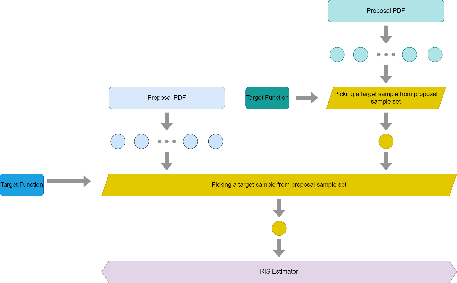
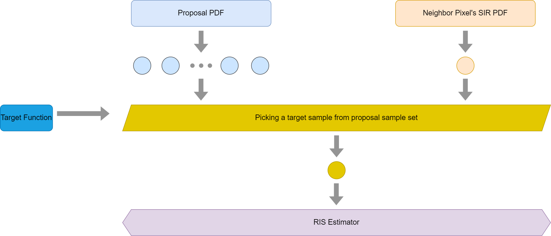
By neighbor sampling, I mean the process to take samples from its neighbors’ reservoirs. I think lots of readers would have confusion similar to mine as well. Since the neighbor pixels don’t share exactly the same target function, there seems no theoretical basis for taking samples from neighbors. The truth is it can take signals from its neighbors and it is also unbiased. In order to understand why, let’s draw a graph first

Let’s observe two pixels, on the left, there is pixel A and on the right, it is pixel B. This graph is about pixel A picking its light samples. In the beginning, both A and B would pick their own proposal samples generated by the light PDF. For pixel A, it would pick neighbors for more signals as well. In this case, let’s assume it picks one of its neighbors, B. Once B is picked, B’s target samples would be fed into A’s weighted reservoir sampling algorithm. And for pixel A, it would use its own target function to pick one winner sample between the winner sample in the proposal light samples that belong to pixel A and the neighbor’s target sample. Eventually, A’s finalized target sample will be fed into the RIS estimator for evaluating rendering equation.

There are a few things I would like to point out in this graph

• For simplicity purposes, this graph is only for the very first frame of rendering with ReStir. Later frames will be more complicated, but they are essentially doing the same thing. It would be a lot easier to understand it once we know how this graph works mathematically.
• Since it is the first frame, there is no temporal reuse as there is no valid history for it to read. Of course, the graph for the whole ReStir DI algorithm would be a bit more complicated.
• Only one neighbor pixel’s reservoir is borrowed in this graph. Borrowing multiple neighbor’s target samples is not essentially different from this one. And the iteration in the neighbor sampling is skipped as well.

With so much simplification, we can still see the complexity of this graph is still beyond the two graphs we showed before. Specifically, how MIS can be used in RIS. If we take a look at the previous two graphs, we would find that it is not immediately obvious if this is MIS + RIS. In order to simplify things, let’s further simplify the graph by taking advantage of the facts of WRS algorithm that were explained before,

• The outcome in WRS is independent of the execution order. It doesn’t matter which proposal sample comes first and the result would be precisely the same.
• Since divide and concur works in WRS as well, it means we can also choose to combine separate WRS executions as well by going the other way around.

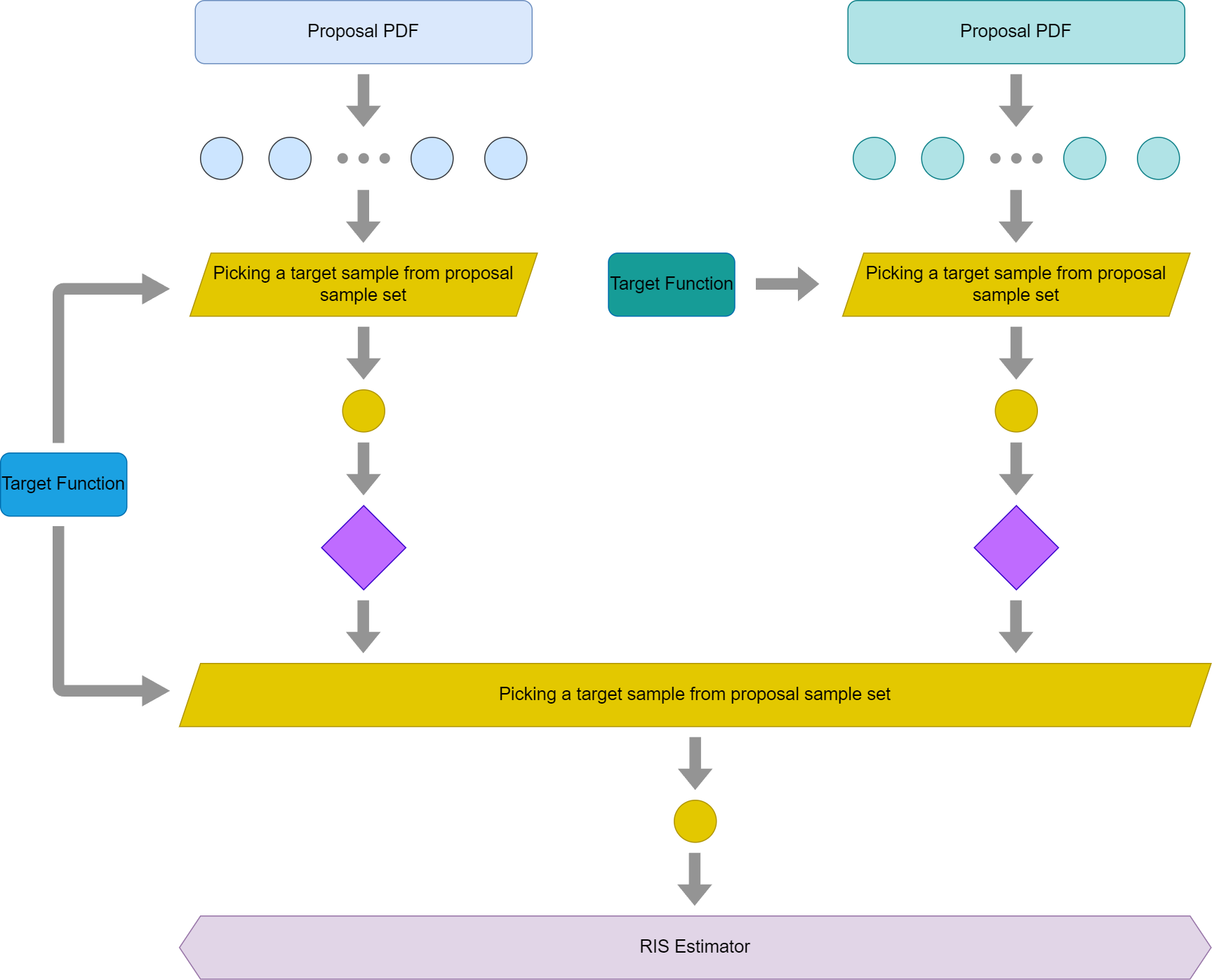
So if we combine the two WRS algorithm execution for pixel A in the previous graph, we would have this new simplified graph then

By observing this graph, it is still not obvious if this is MIS with RIS. But we can quickly notice one important thing here, the target sample generated by neighbor pixel is essentially a SIR algorithm itself. As previously mentioned, SIR is an algorithm that approximates drawing samples from a target pdf. So if we swap the top right corner graph with a single PDF, which is essentially a SIR PDF, we would have this graph then.

Please take a look at the first graph in this section again, I think it should be quite clear that we are essentially just using MIS in RIS. To further explain it, it treats the target sample from its neighbors as a proposal sample here and the proposal PDF for this sample is the SIR PDF from its neighbors. As we mentioned in the previous sections, RIS does allow different proposal PDFs to co-exist together.

At this point, it is clear how we can answer the question of this section. The behavior of borrowing neighbor pixels’ target sample is essentially introducing a new PDF that is different than the light sample PDF. And mathematically this is totally fine and introduces no bias at all as proved before. This is precisely why even if neighbor pixels have their own target functions the algorithm is still unbiased.

One subtle thing that deserves our attention is that ReStir DI really uses different proposal PDFs even if all light samples are drawn from the same light sample PDF. This is because the target samples from neighbors, which are treated as proposal samples, all come from different SIR PDFs.

The Proposal Samples Visited by RIS

One common misunderstanding of ReStir DI algorithm is that if a neighbor pixel’s reservoir has visited 100 samples, by ‘merging’ the target sample from it, our current pixel’s visited samples count will be grown by 100. This was briefly mentioned before, I’d like to explain with a bit more text here.

Let’s keep talking about pixel A and B in the above graph. Except this time, for simplicity, we only pretend that each of them generates two proposal samples. For pixel A, its two proposal samples are $x_0$, $x_1$ and for pixel B, they are $y_0$ and $y_1$.

In order to count the fact that neighbor pixel uses a different target function, the new weight for this target sample of pixel B is

Assuming that pixel B picks $y_0$ as its target sample. If we drop this weight in the SIR sampling execution in the pixel of A during the neighbor sampling phase, we would easily see the final total weight for the pixel A would be

If pixel A visits the four samples by itself, rather than borrowing from its neighbors, the total weight we should see is

This mismatch confused me for quite a while. It doesn’t look like borrowing from neighbor pixel B’s target sample would result in precisely the same math with iterating through B’s proposal samples by itself. My understanding of it is that they are not the same. And please be mindful that I purposely removed the subscript to give us an illusion that all proposal PDFs are the same. Again, even if the light sample PDFs are all consistent across the implementation, the SIR PDF’s presence easily breaks this assumption. So in reality, the above math could be slightly more complicated.

The same theory is hidden in the second graph shown the above section as well. The fact that we used B’s target function can’t be changed by the time A tries to merge B’s target sample. This is no sufficient mathematical proof that pixel A’s reservoir would be able to visit any of the proposal samples of pixel B even if it merges B’s target sample.

Rather than thinking about it that way, I would prefer to think that pixel A would only see its own initial light samples first. For each neighbor sampling, it sees nothing but one single higher quality sample based on a SIR PDF that is a lot closer to the target pdf compared with the light sample proposal PDFs. The more samples visited by neighbor’s reservoir, the higher quality its target sample would be. To some degree, we can think about it this way, pixel A visits pixel B’s proposal samples indirectly, definitely not in a way that regular proposal samples are visited. Of course, this is just an intuitive explanation.

To emphasize it, we need to be aware that by merging neighbor’s target sample it doesn’t give us the mathematical equivalent of visiting neighbor’s light proposal samples. But it does offer a higher quality sample than the initial light samples, which means that we would still benefit a lot if neighbor pixels have visited tons of proposal samples.

What is the MIS Weight?

With the above explanation, I think some readers may have already had a question at this point. What is the MIS weight in this case then? Can we use balance heuristics at all?

There are a few things making the problem a bit tricky,

• The SIR PDF of neighbor’s sampling method is not even tractable. This doesn’t meet the need for balance heuristics in the first place and is a clear deal breaker.
• Assuming there is N samples to be processed, the time complexity for evaluating balance heuristics for all of them will be $O(N^2)$. This may not sound that crazy at the beginning if we only have 32 initial samples along with a few neighbor target samples. Besides the time complexity, there is also storage requirement that will be O(N) as well.
• And since each balanced heuristic weight would require knowing all proposal PDFs during its evaluation, this would mean that the set of proposal PDFs would be known even during the first samples evaluating its MIS weight, breaking the streaming nature of the ReStir algorithm.

At this point, it is not hard to imagine why the paper’s implementation went for a uniform weight as it can easily be isolated out and doesn’t have the problems mentioned above.

However, uniform weight comes at a cost here. As previously explained, the second condition in MIS is not met by the uniform weight. And this is precisely the essential root cause of why ReStir DI would introduce bias. The paper does explain why it is biased, but seeing the same problem from another perspective commonly offers us a bit deeper understanding. And the solution the paper proposed does exactly the method explained metioned in the constant weight section before.

Strictly speaking, there is chances to use balance heuristics by using the target function rather than the intractable SIR PDF. However, even if this tackles the first problem, the two remaining issues could still be a performance bottleneck. Besides, the balanced heuristic commonly requires each PDF to be normalized, while the target function may not necessarily be normalized, which will cause no bias, but inefficiency in terms of convergence rate.

What is the Proposal PDF for Neighbors Target Sample?

In order to perform RIS algorithm, we would need to know the proposal PDF for each incoming proposal sample. However, there is a particularly tricky problem, the neighbor pixel’s SIR PDF is not tractable. There is no easy way to evaluate what the PDF is.

Luckily enough, the paper does explain that the big W, which is shown below, takes the role of reciprocal of SIR PDF,

Here $y$ is the lucky winner sample that was eventually picked through WRS.

To be more mathematical, the expectation of W is precisely the reciprocal of SIR PDF evaluated at the target sample as long as there is no proposal PDF that is zero there. If there is, we can easily avoid bias by adjusting the constant weight as well.

So even if the SIR PDF is intractable, we can indeed know the unbiased approximation of the reciprocal of the SIR PDF once a target sample is drawn. This is a very important property that allows us to merge target sample without introducing bias.

There is one question that needs a bit of clarification. Why can we replace the PDF with this just because the expectation is a match? It is actually not difficult to prove this, let’s assume that there are only K - 1 proposal samples coming from the lights, there is also a Kth proposal sample borrowed from a neighbor.

Importance of Neighbors’ Target Samples

Careful readers at this point may have already realized that the weight for the neighbor target sample I showed above doesn’t match what the paper used, which is $\hat{p}(x) W(x_M) N$. N is the number of visited proposal samples in the neighbor’s reservoir execution, either directly or indirectly. So where does this N fit in the math?

To answer the question, let’s take a look at another question that has not been answered yet. Assuming there is only one neighbor reservoir sampled just like before. In each frame, for each pixel, there is 32 initial light samples. If the neighbor reservoir has visited N samples so far, it is clearly likely to be a higher quality sample than the light samples if N is relatively big. How does the WRS algorithm know? The truth is it may not know. In order to emphasize the importance of neighbor’s target samples, we can choose to feed them into the current pixel N times, with N being the number of proposal samples visited by the neighbor’s reservoir directly and indirectly. So a target sample that is picked from a million proposal samples will be a million times more respected than an initial light sample drawn in the first phase.

Mathematically, the likelihood of picking this sample will clearly be boosted by N times and since we feed it N times, the number of visited proposal samples in this reservoir would need to be bumped by N as well, not 1. However, we don’t really need to feed the neighbor target sample by N times at all, we only need to feed it once, but with the weight scaled by N and bump the visited sample count by N in the current reservoir. This all can be done within O(1) time.

I think it is clear at this point that the $N$ factor in $\hat{p}(x) W(x_M) N$ really is just a scaling factor. It marks how important we thin the sample should be. It is an over-optimistic scaling factor since those $N$ indirectly visisted sample count is the theoritical maximum. In reality, there could be some duplicated signal that reduces the efficiency of the sample.

Below is the algorithm 4 in the original paper,

1
2
3
4
5
6

function combineReservoirs(q, r1, r2, ..., rk)
  Reservoir s
  for r in {r1, r2, ..., rk} do
    s.update(r.y, p_hat(r.y) * r.W * r.M)
  s.M = s1.M + s2.M + ... + sk.M
  s.W = s.w_sum / (p_hat(s.y) * s.M)

Please notice that the 4th line re-update the M of the reservoir even if it is already updated in the update function on the 3rd line already. It actually overrides that. The M is bumped by one in the update function as it assumes the incoming input sample is only one sample. However, as we essentially treat each target sample as it has multiple duplications and feed them multiple times, we would need to update the visited sample count properly.

Temporal Reuse

At this point, it is not hard to guess that the temporal reuse is nothing but a new target sample treated as a proposal sample. The only requirement for keeping the unbiased nature when merging neighbor pixels is correctly counting the denominator, only count the ones with higher than zero probability. So even if the previous frame’s corresponding pixel is not quite accurate, this is not a problem. It would some negative impact on the convergence, but not the unbiasness nature of the algorithm.

Below is a graph looping all processes ReStir DI does for a pixel, though it doesn’t count the repetitive loop of neighbor sampling.

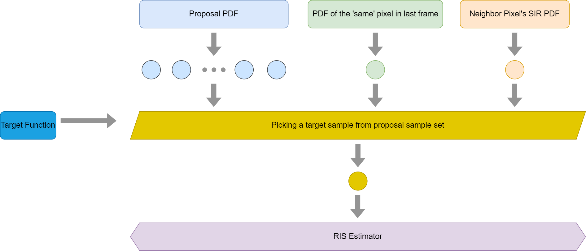
To answer the previous question, why TAA is biased while ReStir temporal reuse is unbiased. In TAA, the lighting signal sampled in the previous frame is already evaluated, which could be incorrect in this frame because of lots of factors, like lighting, animation, occlusion, etc. While in the temporal reuse of ReStir, it only just takes samples, the evaluation hasn’t happened yet. The worst thing that could happen is that it takes a bad sample from some unrelated pixel, but it won’t introduce bias mathematically.

Correcting the Bias in ReStir

In order to correct bias for uniform MIS weight, we would need to evaluate how many PDFs would have non-zero contribution at a specific sample position. Once again, we encounter the same problem as before, the SIR PDF is not tractable.

However, what we need from the SIR PDF is really whether it is large than zero or not, it is a binary information. We don’t really need to know what exactly the value it is. In order to predict that, as we previously mentioned, we can choose to use target function and proposal PDF to predict if SIR PDF is zero. If either of them is zero, the SIR PDF will be zero. On the other hand, if both of them are not zero, the SIR PDF is larger than zero. And we can also take advantage of the fact that any proposal sample positions to be evaluated for bias correction is already on a light source because they originally came in as an initial light sample. Either through direct light proposal PDF or SIR PDF, they indeed made it this far, meaning their proposal PDF is already larger than zero. So all we need to do is to test if the target function is larger than zero or now, which is exactly what the paper does.

Visibility Reuse

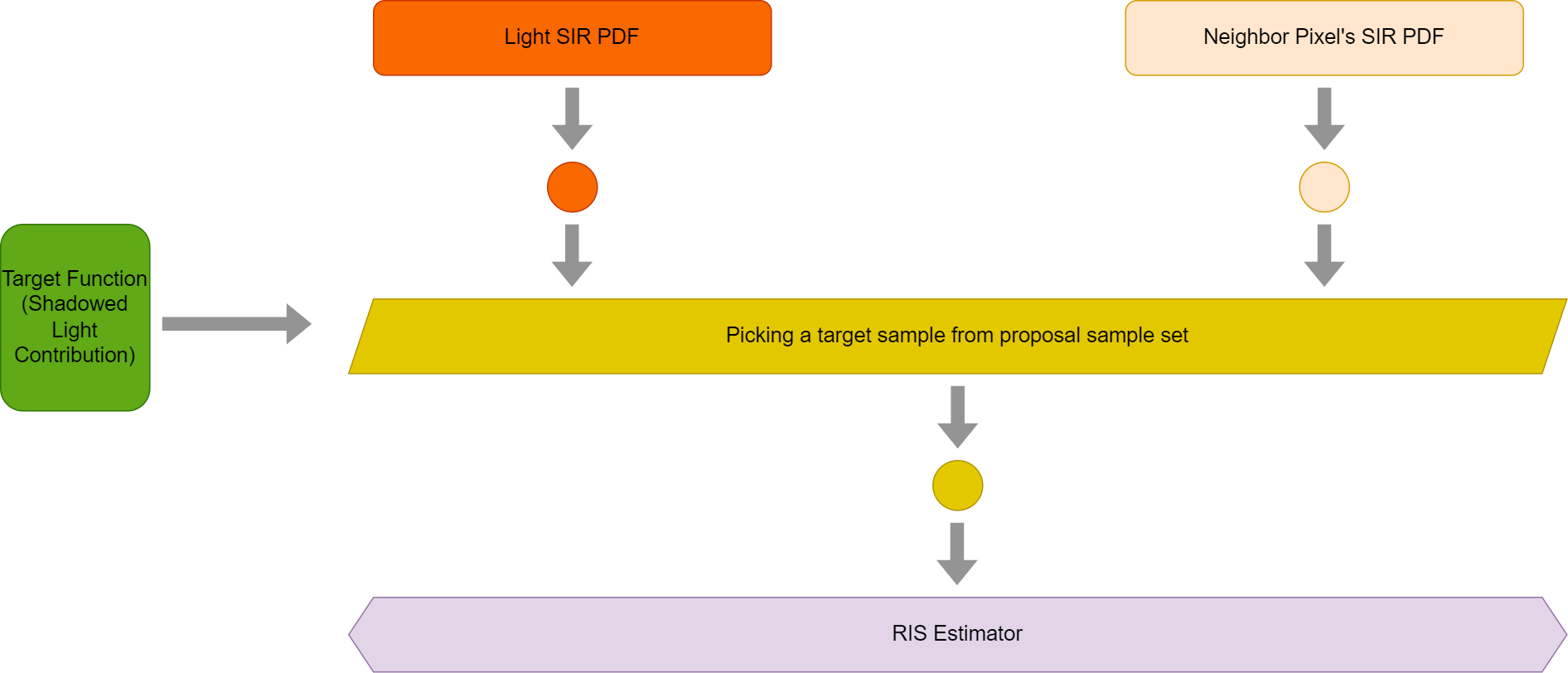
This is the last topic I would like to explain. I almost had myself convinced it was a biased solution for quite a while until recently when I realized it is not. To begin with, let’s start with this graph,

Compared with the first ReStir graph we showed, this simply adds a visibility check (purple diamond shape) before even merging the samples. If it is occluded, it would ignore this sample. If we regard the visibility to be part of the target function, we would simplify the graph this way

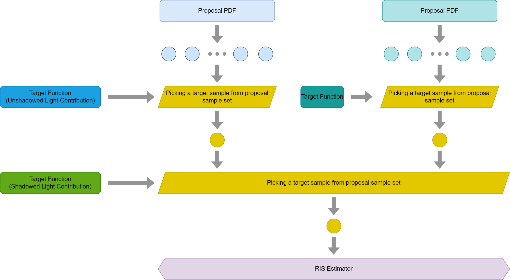
As a matter of fact, RIS does allow per-initial sample target function. So using different target functions for the current pixel in RIS is not a big concern. However, I’d like to explain the theory through another way by pretending that RIS doesn’t allow per-initial sample target function.

For the top left part of the graph, for quite a while, I thought the algorithm should have checked visibilitiy for each proposal light sample, rather than only the winner light sample to make sure the target function is consistent for this pixel’s RIS algorithm.

However, it turns out that we don’t necessarily need to do it even if it is not a wrong thing to do. Just like we regard the whole top right part as a single execution of RIS. We could think about the light samples exactly the same way. One way to understand it is that the current pixel’s reservoir never sees the individual light proposal samples when visibility reuse is used, it sees a target sample drawn from a SIR method with unshadowed light contribution as target function. Just like a neighbor target sample is drawn from a different target function, this simply uses another target function for its own mini RIS execution.

With this explanation, the above graph boils down to this simplified form that we are very familiar with

Needless to explain at this point, this is just MIS used in RIS, something we have visited a few times in this blog. The key observation here is that with visibility reuse, the current pixel’s reservoir no longer sees the light proposal samples anymore and this is why we can use different a target function to filter samples as the later RIS execution sees only one sample drawn from a SIR method, it doesn’t care what target function it uses.

Now we can see that this has its theoretical basis that it is not biased. But we have another follow-up question here, since this is just like sampling a neighbor target sample, we would need to have one single target sample with the proper weight coming in. So if we would like to take a sample from a RIS pdf, we would need to use the weight of $\hat{p}’(x) W(x) N$, where N is the number of light proposal samples and $\hat{p}’(x)$ is the shadowed light contribution $L(w_i) f_r(w_i, w_o) cos(\theta_i) V(p, p’)$, W is just the big W we talked about before. It seems that a more self-explanatory implementation is to use one reservoir to pick light sample winners and another empty reservoir to merge all the target samples, either from light sample filtering, temporal reuse or neighbor pixels’ reservoir. However, rather than starting with a new reservoir in the temporal reuse phase, the paper reuses the light samples reservoir directly, which doesn’t match the graph we showed above. The only thing that the paper does is to adjust the reservoir big W to zero if the winner light sample is occluded. This reuse of reservoir easily gives people an impression that the current pixel’s reservoir has visited all the light proposal samples directly and then the neighbor’s target sample as they seem sharing the same reservoir. The truth is the paper does nothing wrong, so let’s see what happens.

Right after phase 1, where we finished all proposal sample generation and resolved a winner light sample, the current pixel’s reservoir state is

• y -> The selected winner sample.
• $w_{sum}$ -> The sum of all light samples’ weights. Please be noted that the light sample weight’s nominator uses the unshadowed target function, rather than the shadowed one we will use to pick a final sample for this pixel.
• N -> The number of direct light proposal samples it has visited so far. (The paper used M here, in order to stay consistent with my previous derivation, N is used here. It is the same thing.)
• W -> This is a derived member that merely serves as a cache. It doesn’t have any extra signal.

As a reminder, the big W is defined as

Please be noted that I swapped the notation of x and y here, but it is the same thing, except that x is a subset of y now. And M is swapped with N as well. None of these changes the essential meaning of this equation. One subtle change I made here is the lack of subscripts in proposal PDF, this is fine as the paper does indicate it only uses one single proposal PDF for light sample picking, which we have explained as well.

If we would start with a brand new empty reservoir, we would need to treat the resolved target light sample with this weight, $\hat{p}’(x) W(x) N$. Since the new target function is nothing but the original unshadowed target function with an extra binary signal on top of it. We have

If we combine the two math equations and drop a new sample generated by SIR method in an empty reservoir, we would have this as its weight for the incoming proposal sample in the execution of this pixel’s RIS execution,

So if we would start from a new reservoir, the weight for the one single sample, which is the resolved target light sample, is exactly the sum of all previous light samples’ weight, but with an extra visibility term. Please be mindful that the nominator in the sum is the original unshadowed target function, rather than the new shadowed one.

Depending on the occlusion situation, we have two possibilities here,

• If the resolved light target sample is not occluded, we have precisely what is already cached in the reservoir after phase 1.
• If it is occluded, this single new sample will have zero weight as its target function is zero. All we need to do is to adjust the weight to zero, which is exactly what the paper does.

It is a lot easier to understand the other members in the reservoir data structure,

• For the picked sample, regardless which of the two implementations is used, after the optional phase, they all pick the resolved light sample. Of course, if it is occluded, nothing is picked.
• And for the number of visited samples in the reservoir, since we pretend to duplicate the resolved light target sample by the number of visited proposal light samples, this is a perfect match as well.
• Since the big W is nothing but a cache, it is also a match as all its variables are already matched.

So now we can see that the paper does indeed implement the same thing if we take a deeper look at the math. Hopefully, this would convince readers that this algorithm is indeed unbiased.

Summary

In this blog post, I summarized my understanding of the original ReStir algorithm. I dug into the mathematical details and explained why the algorithm is unbiased. This blog is what I collected during my learning process. I put it down here in the hope that it could be helpful to those people who have similar confusion like myself. Hopefully, this could be helpful for someone to get a deeper understanding of the tech.

This blog doesn’t mention any engineering problems that we could face during implementing ReStir, like memory cache issue when sampling millions of lights, floating point precision overflow issue after a few iterations, etc. For more details about that part, I would recommend watching this talk or taking a look at the source code of RTX DI.

Reference

[1] Spatiotemporal reservoir resampling for real-time ray tracing with dynamic direct lighting
[2] ReSTIR GI: Path Resampling for Real-Time Path Tracing
[3] Generalized Resampled Importance Sampling: Foundations of ReSTIR
[4] Fast Volume Rendering with Spatiotemporal Reservoir Resampling
[5] How to add thousands of lights to your renderer and not die in the process
[6] Spatiotemporal Reservoir Resampling (ReSTIR) - Theory and Basic Implementation
[7] Robust Monte Carlo Methods For Light Transport Simulation
[8] Practical implementation of MIS in Bidirectional Path Tracing
[9] Importance Resampling for Global Illumination
[10] Sampling Importance Resampling
[11] Monte Carlo Integral with Multiple Importance Sampling
[12] Dynamic Many-Light Sampling for Real-Time Ray Tracing
[13] Importance Sampling of Many Lights with Adaptive Tree Splitting
[14] Rendering Many Lights With Grid-Based Reservoirs
[15] High Quality Temporal SuperSampling
[16] Physically Based Rendering
[17] Sampling Importance Resampling (blog)
[18] Picking Fairly From a List of Unknown Size With Reservoir Sampling
[19] Rendering Games With Millions of Ray-Traced Lights
[20] Light Resampling In Practice with RTXDI
[21] Global illumination overview in Kajiya Renderer
[22] RTXDI: Details on Achieving Real-Time Performance
[23] Rearchitecting Spatiotemporal Resampling for Production