I posted a blog about path tracing some time ago, I didn’t regard it as a simple algorithm until I got my hands dirty on bidirectional path tracing. It really took me quite a while to get everything hooked up. Getting BDPT (short for bidirectional path tracing) converging to the same result with path tracing is far from a trivial task, any tiny bug hidden in the renderer will drag you into a nightmare. Those kind of bugs are not the same with the ones that usually appear in real time rendering, like the ones that can easily be exposed with some tools like Nsight, it may cost much more time if only a small component is missing in the target equations, which are totally crazy math.

Since traditional cornell box setting is pretty friendly to path tracing, I made a little change on it, the light source is a spot light facing towards right up. That said most of the scene is lit by the small direct illuminated area instead of the light, that just makes it a very unfriendly path tracing scene.

The following images are generated by BDPT(left), light tracing(middle) and path tracing(right) with roughly the same amount of time.

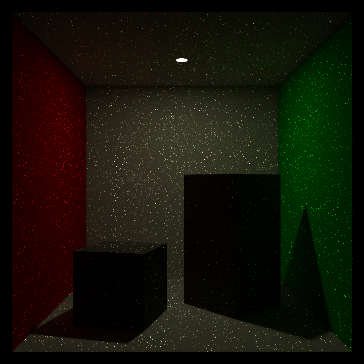
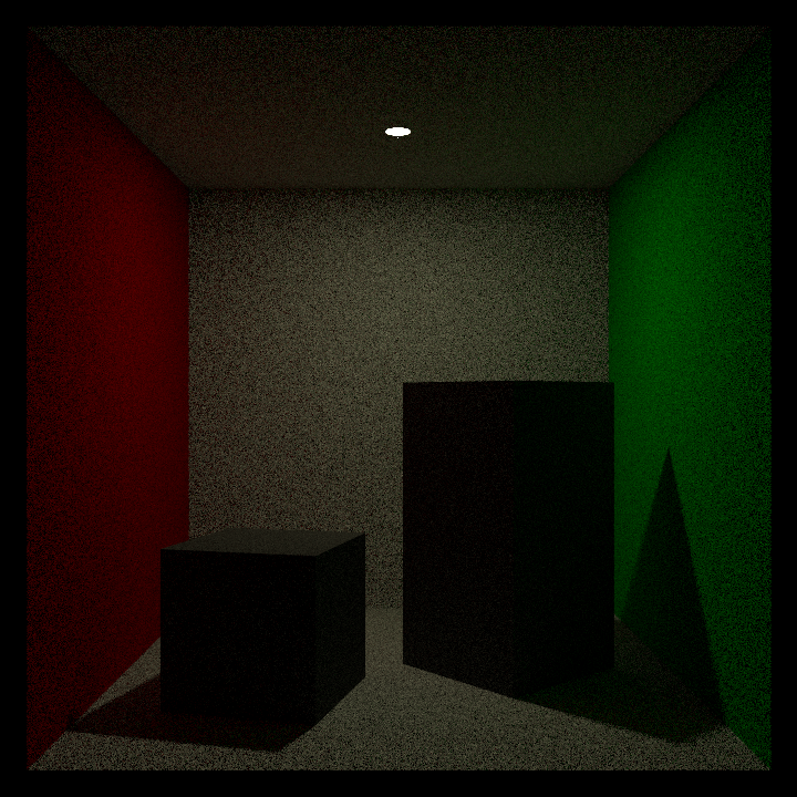
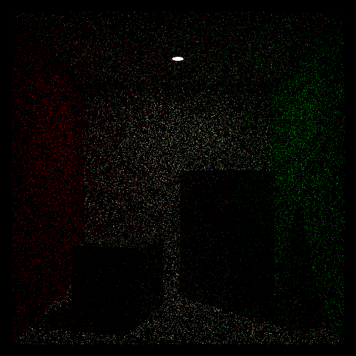
Path tracing generates the most noisy image even if it is scaled down by four times, bidirectional path tracing result is better, however light tracing definitely gets the best result with least noise in it.

Rendering Equation

Starting from rendering equation:

$$ {L_{o}(\omega_{o}) = L_{e}(\omega_{o}) + \int L_{i}(\omega_{i}) *f( \omega_{i}, \omega_{o} ) *cos(\theta_{i}) d\omega_{i}} $$

As we can see from this classical equation, L appears at both sides of the equation which makes it a recursive one. By expending this equation for a specific path, we will have something like this:

$$ f_k(x) = {\int...\int} W_e(x_0) G(x_0 \longleftrightarrow x_1 ) [ \prod_{i=1}^{k-1} \rho_s(x_i)G(x_i\longleftrightarrow x_{i+1} ) ] L_e(x_k) d(x_0) d(x_1) ... d(x_k) $$

That is the equation considering a specific path with length of k+1 vertices between light and eye. Starting from where is really a matter of taste, traditional path tracing generates rays from eye point. Light tracing tries to solve it in a manner that is more similar to how nature works, generating rays from light. Bidirectional path tracing generates rays from both sides and connects those two path somehow.

Path tracing

I’ve talked about path tracing in this blog, those path are generated with regard to the bsdf. This time we will put it the other way. Since we already have the equation to be integrated, we only need to know the pdf of the specific path to evaluate the integral with Monte Carlo method.

Suppose all of the vertices are generated w.r.t the area instead of solid angle, we have a pdf of this:

$$ p_k(x) = \prod_{i=0}^{k} p_a(x_i) $$

However generating vertices in this manner is extremely inefficient and it is no path tracing we are talking about. A path tracer generates rays from eye point recursively. Forget about the aperture with finite size. The first vertex apart from the camera one is already decided by the camera, so no pdf is needed here. Each of the others will be generated based on the pdf w.r.t (projected) solid angle, we have a relationship between them:

$$ p_a(x_i) = p_{w^{\bot}}(x_{i-2} \rightarrow x_{i-1} \rightarrow x_i) G(x_{i-1}\longleftrightarrow x_i ) $$

Dropping this into the P_k equation, we will have this:

$$ p_k(x) = \prod_{i=2}^{k}(p_{w^{\bot}}(x_{i-2} \rightarrow x_{i-1} \rightarrow x_i) G(x_{i-1}\longleftrightarrow x_i )) $$

Also filling this into the extended rendering equation, we will have something like this:

$$ f(x)=L_e(x_k\rightarrow x_{k-1})\prod_{i=2}^{k}(bxdf(x_{i-2}\rightarrow x_{i-1}\rightarrow x_i)/p_{w^{\bot}}(x_{i-2} \rightarrow x_{i-1} \rightarrow x_i))$$

We have less computation here because the g term has been cancelled with the components in the denominator.

In a real practical path tracer, we usually use multiple importance sampling to sample both bsdf and light sources at the end of each path, instead of relying on bsdf alone which is highly inefficient for small light sources. The pdf may need to change correspondingly.

One minor detail that used to confuse me so far is where is the g-term connecting the first vertex and eye point going? Why don’t we take the pdf of primary ray into account? Please refer to this post for an explanation.

Light Tracing

Light tracing is the reverse version of path tracing. Instead of starting from the eye point, light tracing path origins from light sources. For a path tracer, it may be acceptable without special handling with MIS sampling both bsdf and light sources if light sources are big enough. However light tracing must connect light path vertices to the camera point explicitly, even if light aperture has a size in the scene, its small area will make light tracing converging in an extreme slow manner.

Similarly we have the pdf of a specific light path in the following way:

$$ p_k(x)=p_a(x_k)p_{w^\bot}(x_k\rightarrow x_{k-1})G(x_k\rightarrow x_{k-1})\prod_{i=3}^{k}(p_{w^{\bot}}(x_{i}\rightarrow x_{i-1}\rightarrow x_{i-2})G(x_{i-1}\rightarrow x_{i-2})$$

Note that it is only part of the whole pdf, because we haven’t consider eye vertex yet. As I mentioned above, in a light tracing algorithm we usually connect eye vertex with light tracing vertices as we progress in the light path, trying to hit the camera aperture with light rays is just not practical, not to mention it won’t work for pinhole camera at all.

To connect eye point with light tracing vertices, we need to be clear with the importance function. For a detailed description of how to calculate it, I suggest my other post.

Although we can make the path contribute to the pixel we are trying to calculate, it is very inefficient way of doing light tracing because most path will fail resulting into an extreme slow convergence rate. Instead, we usually allow all path to contribute to any pixels in the target image we are rendering.

And light tracing achieves the best result out of the three method in the above comparison for a reason, the spot light change makes the scene pretty light tracing friendly because basically all light paths contribute to the image.

Bidirectional Path Tracing

Different from unidirectional path tracing, bidirectional path tracing generates path from both light sources and eye point and then combines each pair of vertices at two sides, including the traditional path tracing path and light tracing path. In some sense that bidirectional path tracing is a super set of path tracing and light tracing.

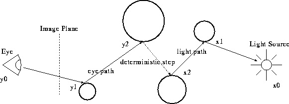
Here is a great demonstration from Eric Veach’s thesis. For a specific length of three, we have four cases above. The first two cases are what we usually do in path tracing, the third one is the light tracing we are talking about. The last one is the case when light ray actually hits the aperture and in most cases we just ignore the fourth case because it brings no differentiation comparing with the third case.

Each case is good at rendering something. If the surface of the table is highly reflective, in other words with spiky brdf, the first case will generate the best result. However if the light source is very small or delta light source, like point light, and the table surface gets a matte look, the second one will be much better. Light tracing case may not be very powerful in this very case, however if there were some glasses, light tracing will deliver good looking caustics in an efficient manner.

Since we’ve already talked about the first three cases, I’d like to mention another case which is not shown in the above image.

I won’t write down the equation here because it is pretty similar to the ones mentioned above. However one noticeable detail is that we missed one g-term in the denominator, it is the g-term between the connecting vertices that can’t be cancelled, we need to evaluate the g-term explicitly in this case, or the result will be biased.

By combining all those cases, except the last one, we will get rich information from all paths we generated. A naive implementation is to average all those results of paths with specific length. For example, the averaging factor of five vertices path (including the light and eye vertex) is 1/5.

Further Work

As you can see from the top image, that BDPT generates noisy images than light tracing in the target scene. Sometimes it is worse than path tracing depending on what kind of scene it renders.

Multiple importance sampling can solve this disturbing issue and that is what I’m going to work on, :).

Reference

[1] Robust Monte Carlo Methods For Light Transport Simulation. Eric Veach
[2] Small VCM renderer
[3] Calculating the directional probability of primary rays
[4] Bidirectional path tracing
[5] Wonderball