Image-based lighting is a practical way to enhance the visual quality of computer graphics. I used to be confused by it until I read the book “High Dynamic Range Imaging”, which provides a very clear explanation about IBL. And I actually have implemented the algorithm in my offline renderer before, it was just that I didn’t know it is IBL. The book PBRT has some materials talking about it without explicitly mentioning the term. Following images are generated with IBL in my renderer, except that the last one uses a single directional light.

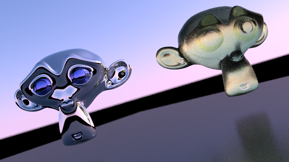
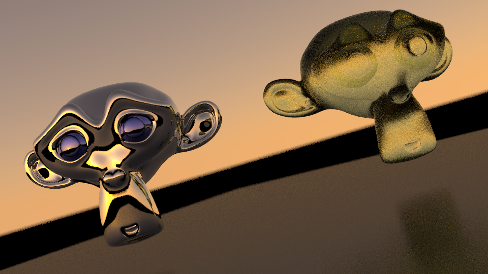
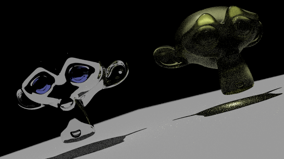
As we can see from the above images, IBL generated images looks way more promising than the one with a directional light. The real beauty of it is that with physically based shading everything looks great in different lighting environments without the need to change material parameters at all.

IBL in Offline Rendering

Unlike IBL in real-time rendering, offline ray tracers can easily achieve unbiased result with IBL without compromising anything. The techs involved in generating the above images are introduced in my previous blogs, like path tracing, Monte-Carlo Integration, Importance sampling for microfacet BRDF. I won’t repeat them again in this blog.

First thing first, what is image based lighting. My take on it is that IBL uses a special HDR map recording all incoming radiance from different solid angles to simulate complex lighting environment. It is pretty much like the spherical reflection map we used to render reflective materials in the old days. For old-school reflective materials in real time rendering, only one texture sampling is necessary, which makes the algorithm feasible even in fixed function pipe. Since not all materials need only one texture sampling, using the HDR image to render other materials is a challenging task. The essential difference between the two lies in the fact that pure reflective BRDF is actually delta function, which will reduce the dimension of the integral. In offline rendering, since speed is not the most sensitive thing, one can always use Monte-Carlo method to evaluate the integral of rendering equation. So, in a nut-shell, IBL is a technique that uses HDR environment light to light 3d objects in the scene.

Below is an HDR image used in the first images shown above. Of course, it has been converted into LDR since majority displays on the market doesn’t support HDR.

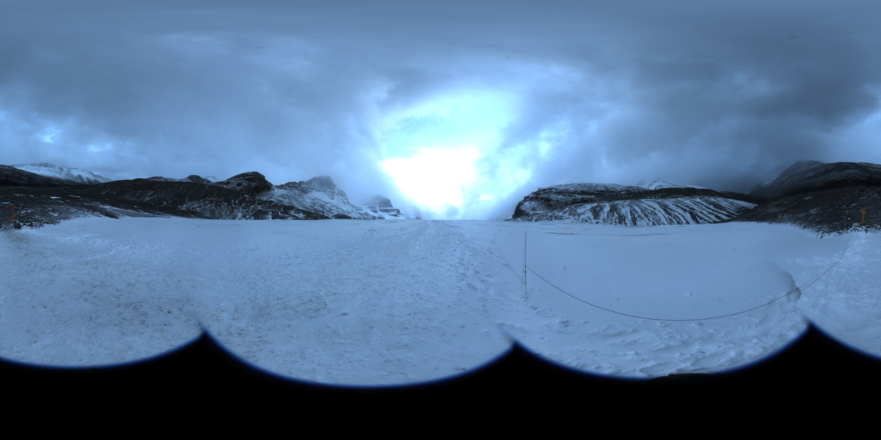
The only important thing that is not mentioned in my previous blog is how to do importance sampling with the HDR image. It is actually quite simple, just a discretized inversion method. Please refer to the book PBRT for further detail implementation of it.

IBL in Real Time Rending (UE4 implementation)

UE4’s implementation of IBL is really impressive. Usually, 1024 samples may be needed to generate a noise-free image. However, 1024 times sampling is nothing practical in a real-time rendering engine, it will make the rendering application heavily bandwidth bounded. UE4 uses a tricky way to resolve the issue of the excessive number of samplings, reducing it from a thousand to two samplings and making IBL a practical algorithm in it. Of course, it is an estimation of the rendering equation. That said it is far from unbiased. However, truth is there are biases everywhere in real time rendering, one extra source of bias doesn’t even hurt at all.

The slide is here. However, one can easily get lost like I did during the introduction of IBL in this slide. Luckily, the note explains everything in a very clear manner.

Split Sum Approximation

I will skip the original rendering equation and its Monte Carlo integration. We need to evaluate the following equation in a very efficient manner.

$$ \dfrac{1}{N} \sum_{k=1}^{N} \dfrac{L_i(l_k) f(l_k,v) cos\theta_{l_k}}{p(l_k,v)} \approx (\dfrac{1}{N} \sum_{k=1}^{N} L_i(l_k) ) (\dfrac{1}{N} \sum_{k=1}^{N} \dfrac{f(l_k,v) cos\theta_{l_k}}{p(l_k,v)} ) $$

The approximation is not exactly 100% accurate. However, the bias introduced in a real rendering scene can be barely noticed.

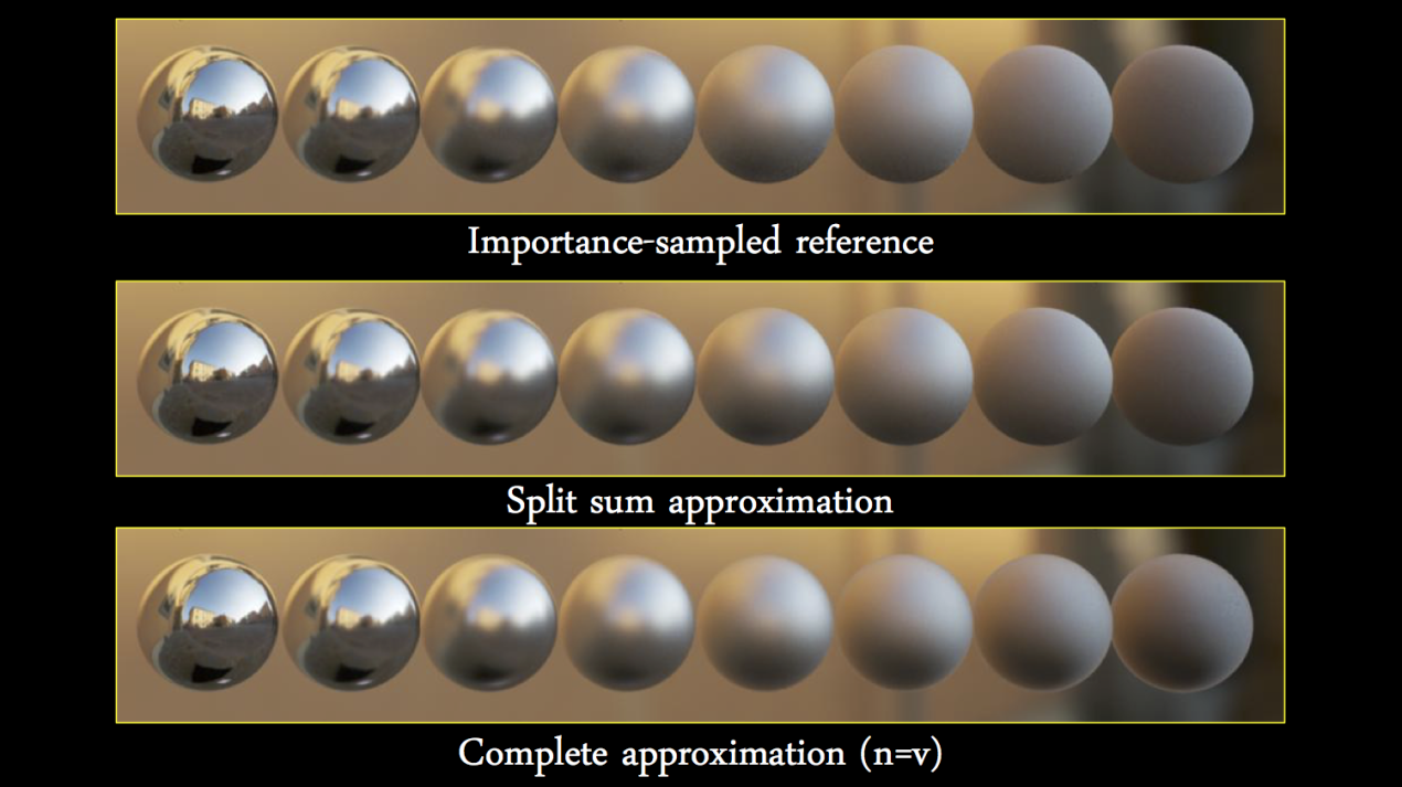
The above slide comes from UE4’s presentation in Siggraph 2013, I can barely tell the difference between the balls in the first two rows. Clearly, the split sum is an acceptable approximation in real time rendering. However, the goal here is to reduce the number of sampling in IBL tech, splitting the equation is only the beginning, it doesn’t reduce anything yet at all. The golden idea here is to pre-compute some computation heavy task first before real-time rendering happens.

Pre-Filter Environment Map

Following is the first part of the split sum, it is relatively easy to pre-compute an estimation.

$$ \dfrac{1}{N} \sum_{k=1}^{N} L_i(l_k) $$

Averaging the radiance for different roughness will yield a good result and we can actually store textures for each roughness value into different mipmap levels. However, UE4 convolves the environment map with the GGX distribution of their shading model using importance sampling. One minor detail is that since microfacet BRDF is also a function of incoming angle, they actually made an assumption that the incoming angle is actually zero, in other words, the incoming direction is exactly the opposite of the surface normal. Of course, it introduces another source of bias here.

Environment BRDF

This is actually where the most magic happens. Let’s first look at the original integral form of the equation.

$$ \int_H f(w_i,w_o) cos\theta_{w_i} dw_i $$

By assuming the BRDF is actually microfacet model, we have the form of BRDF like this:

$$ f(\omega_i,\omega_o,x) = \dfrac{F(\omega_i , h) G(\omega_i,\omega_o,h) D(h)}{4 cos(\theta_i) cos(\theta_o)} $$

Schlick’s approximation of Fresnel is used in it:

$$ F(w_i,h) = F_0 + ( 1 - F_0 ) ( 1 - w_i h )^5 $$

In order to pre-compute what we need in shading, we need to know how many parameters there are in the BRDF. The obvious ones are the incoming direction, outgoing direction, roughness, albedo (or direction-hemisphere reflectance). Since what we care is how to compute the integral efficiently, the incoming direction is not our concern at all, leaving us five dimensions, out going direction, roughness and albedo ( three dimensions here because it is a color ). One may wonder here that isn’t outgoing direction two-dimensional? The truth is only the cosine factor of the angle between it and the normal is relevant in a D-term, thus reducing it to one single dimension. Sadly a five dimensional data is really hard to pre-computed before-hand.

As a matter of fact, a simple math trick will factor albedo out of the equation:

$$ \int_H f(w_i,w_o) cos\theta_{w_i} dw_i = F_0 \int_H \frac{f(w_i,w_o) cos\theta_{w_i}}{F( w_i, h )} ( 1 - ( 1 - w_i h )^5 ) d w_i +\int_H \frac{f(w_i,w_o) cos\theta_{w_i}}{F( w_i, h )} ( 1 - w_i h )^5 d w_i $$

Don’t be scared by the complex equation, it is actually clearer than it used to be before. Now, we only need to evaluate the first and second integral on the right side before-hand, leaving the F0 or albedo evaluation in the real time rendering.

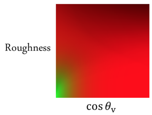
With only two dimensions in the equation, we can save the pre-computed information in one single texture. And the above texture is one example of it. During pixel shading, one can simply estimate the integral with the following calculation:

$$ EnvBRDF = Color * tex2d( cos\theta_o , roughness ).x + tex2d( cos\theta_o , roughness ).y $$

It looks simpler enough to me. Only one texture sampling to evaluate the second integral of the split sum!

Above is a comparison between the reference, split sum and the simplified method in real time rendering. Pretty cool approximation.

Reference

[1] High Dynamic Range Imaging
[2] Real Shading in UE4
[3] Physically Based Shading